The aim of air pollution modelling is the estimation of outdoor pollutant concentrations caused, for instance, by industrial production processes, accidental releases or traffic. Air pollution modelling is used to ascertain the total concentration of a pollutant, as well as to find the cause of extraordinary high levels. For projects in the planning stage, the additional contribution to the existing burden can be estimated in advance, and emission conditions may be optimized.

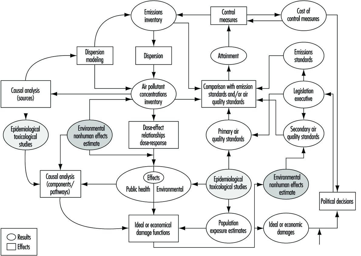
Figure 1. Global Environmental Monitoring System/Air pollution management

Depending on the air quality standards defined for the pollutant in question, annual mean values or short-time peak concentrations are of interest. Usually concentrations have to be determined where people are active - that is, near the surface at a height of about two metres above the ground.

Parameters Influencing Pollutant Dispersion

Two types of parameters influence pollutant dispersion: source parameters and meteorological parameters. For source parameters, concentrations are proportional to the amount of pollutant which is emitted. If dust is concerned, the particle diameter has to be known to determine sedimentation and deposition of the material (VDI 1992). As surface concentrations are lower with greater stack height, this parameter also has to be known. In addition, concentrations depend on the total amount of the exhaust gas, as well as on its temperature and velocity. If the temperature of the exhaust gas exceeds the temperature of the surrounding air, the gas will be subject to thermal buoyancy. Its exhaust velocity, which can be calculated from the inner stack diameter and the exhaust gas volume, will cause a dynamic momentum buoyancy. Empirical formulae may be used to describe these features (VDI 1985; Venkatram and Wyngaard 1988). It has to be stressed that it is not the mass of the pollutant in question but that of the total gas that is responsible for the thermal and dynamic momentum buoyancy.

Meteorological parameters which influence pollutant dispersion are wind speed and direction, as well as vertical thermal stratification. The pollutant concentration is proportional to the reciprocal of wind speed. This is mainly due to the accelerated transport. Moreover, turbulent mixing increases with growing wind speed. As so-called inversions (i.e., situations where temperature is increasing with height) hinder turbulent mixing, maximum surface concentrations are observed during highly stable stratification. On the contrary, convective situations intensify vertical mixing and therefore show the lowest concentration values.

Air quality standards - for example, annual mean values or 98 percentiles - are usually based on statistics. Hence, time series data for the relevant meteorological parameters are needed. Ideally, statistics should be based on ten years of observation. If only shorter time series are available, it should be ascertained that they are representative for a longer period. This can be done, for example, by analysis of longer time series from other observations sites.

The meteorological time series used also has to be representative of the site considered - that is, it must reflect the local characteristics. This is specially important concerning air quality standards based on peak fractions of the distribution, like 98 percentiles. If no such time series is at hand, a meteorological flow model may be used to calculate one from other data, as will be described below.

The Global Atmospheric Watch (GAW) programme (Miller and Soudine 1994) provides data and other information on the chemical composition and related physical characteristics of the atmosphere, and their trends, with the objective of understanding the relationship between changing atmospheric composition and changes of global and regional climate, the long-range atmospheric transport and deposition of potentially harmful substances over terrestrial, fresh-water and marine ecosystems, and the natural cycling of chemical elements in the global atmosphere/ocean/biosphere system, and anthropogenic impacts thereon. The GAW programme consists of four activity areas: the Global Ozone Observing System (GO3OS), global monitoring of background atmospheric composition, including the Background Air Pollution Monitoring Network (BAPMoN); dispersion, transport, chemical transformation and deposition of atmospheric pollutants over land and sea on different time and space scales; exchange of pollutants between the atmosphere and other environmental compartments; and integrated monitoring. One of the most important aspects of the GAW is the establishment of Quality Assurance Science Activity Centres to oversee the quality of the data produced under GAW.

Concepts of Air Pollution Modelling

As mentioned above, dispersion of pollutants is dependent on emission conditions, transport and turbulent mixing. Using the full equation which describes these features is called Eulerian dispersion modelling (Pielke 1984). By this approach, gains and losses of the pollutant in question have to be determined at every point on an imaginary spatial grid and in distinct time steps. As this method is very complex and computer time consuming, it usually cannot be handled routinely. However, for many applications, it may be simplified using the following assumptions:

• no change of emission conditions with time

• no change of meteorological conditions during transport

• wind speeds above 1 m/s.

In this case, the equation mentioned above can be solved analytically. The resulting formula describes a plume with Gaussian concentration distribution, the so called Gaussian plume model (VDI 1992). The distribution parameters depend on meteorological conditions and downwind distance as well as on stack height. They have to be determined empirically (Venkatram and Wyngaard 1988). Situations where emissions and/or meteorological parameters vary by a considerable amount in time and/or space may be described by the Gaussian puff model (VDI 1994). Under this approach, distinct puffs are emitted in fixed time steps, each following its own path according to the current meteorological conditions. On its way, each puff grows according to turbulent mixing. Parameters describing this growth, again, have to be determined from empirical data (Venkatram and Wyngaard 1988). It has to be stressed, however, that to achieve this objective, input parameters must be available with the necessary resolution in time and/or space.

Concerning accidental releases or single case studies, a Lagrangian or particle model (VDI Guideline 3945, Part 3) is recommended. The concept thereby is to calculate the paths of many particles, each of which represents a fixed amount of the pollutant in question. The individual paths are composed of transport by the mean wind and of stochastic disturbances. Due to the stochastic part, the paths do not fully agree, but depict the mixture by turbulence. In principle, Lagrangian models are capable of considering complex meteorological conditions - in particular, wind and turbulence; fields calculated by flow models described below can be used for Lagrangian dispersion modelling.

Dispersion Modelling in Complex Terrain

If pollutant concentrations have to be determined in structured terrain, it may be necessary to include topographic effects on pollutant dispersion in modelling. Such effects are, for example, transport following the topographic structure, or thermal wind systems like sea breezes or mountain winds, which change wind direction in the course of the day.

If such effects take place on a scale much larger than the model area, the influence may be considered by using meteorological data which reflect the local characteristics. If no such data are available, the three-dimensional structure impressed on the flow by topography can be obtained by using a corresponding flow model. Based on these data, dispersion modelling itself may be carried out assuming horizontal homogeneity as described above in the case of the Gaussian plume model. However, in situations where wind conditions change significantly inside the model area, dispersion modelling itself has to consider the three-dimensional flow affected by the topographic structure. As mentioned above, this may be done by using a Gaussian puff or a Lagrangian model. Another way is to perform the more complex Eulerian modelling.

To determine wind direction in accord with the topographically structured terrain, mass consistent or diagnostic flow modelling may be used (Pielke 1984). Using this approach, the flow is fitted to topography by varying the initial values as little as possible and by keeping its mass consistent. As this is an approach which leads to quick results, it may also be used to calculate wind statistics for a certain site if no observations are available. To do this, geostrophic wind statistics (i.e., upper air data from rawinsondes) are used.

If, however, thermal wind systems have to be considered in more detail, so called prognostic models have to be used. Depending on the scale and the steepness of the model area, a hydrostatic, or the even more complex non-hydrostatic, approach is suitable (VDI 1981). Models of this type need much computer power, as well as much experience in application. Determination of concentrations based on annual means, in general, are not possible with these models. Instead, worst case studies can be performed by considering only one wind direction and those wind speed and stratification parameters which result in the highest surface concentration values. If those worst case values do not exceed air quality standards, more detailed studies are not necessary.

Figure 2. Topographic structure of a model region

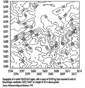
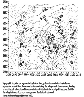
Figure 2, figure 3 and figure 4 demonstrate how the transport and dispension of pollutants can be presented in relation to the influence of terrain and wind climatologies derived from consideration of surface and geostrophic wind frequencies.

Figure 3. Surface frequency distributions as determined from geostrophic  frequency distribution

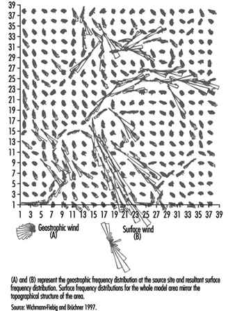
Figure 4.  Annual mean pollutant concentrations for a hypothetical region calculated  from the geostrophic frequency distribution for heterogeneous wind fields

Dispersion Modelling in Case of Low Sources

Considering air pollution caused by low sources (i.e., stack heights on the order of building height or emissions of road traffic) the influence of the surrounding buildings has to be considered. Road traffic emissions will be trapped to a certain amount in street canyons. Empirical formulations have been found to describe this (Yamartino and Wiegand 1986).

Pollutants emitted from a low stack situated on a building will be captured in the circulation on the lee side of the building. The extent of this lee circulation depends on the height and width of the building, as well as on wind speed. Therefore, simplified approaches to describe pollutant dispersion in such a case, based solely on the height of a building, are not generally valid. The vertical and horizontal extent of the lee circulation has been obtained from wind tunnel studies (Hosker 1985) and can be implemented in mass consistent diagnostic models. As soon as the flow field has been determined, it can be used to calculate the transport and turbulent mixing of the pollutant emitted. This can be done by Lagrangian or Eulerian dispersion modelling.

More detailed studies - concerning accidental releases, for instance - can be performed only by using non-hydrostatic flow and dispersion models instead of a diagnostic approach. As this, in general, demands high computer power, a worst case approach as described above is recommended in advance of a complete statistical modelling.

Back