This article is intended to provide the reader with an understanding of currently available technology for approaching water pollution control, building on the discussion of trends and occurrence provided by Hespanhol and Helmer in the chapter Environmental Health Hazards. The following sections address the control of water pollution problems, first under the heading “Surface Water Pollution Control” and then under the heading “Groundwater Pollution Control”.

Surface Water Pollution Control

Definition of water pollution

Water pollution refers to the qualitative state of impurity or uncleanliness in hydrologic waters of a certain region, such as a watershed. It results from an occurrence or process which causes a reduction in the utility of the earth’s waters, especially as related to human health and environmental effects. The pollution process stresses the loss of purity through contamination, which further implies intrusion by or contact with an outside source as the cause. The term tainted is applied to extremely low levels of water pollution, as in their initial corruption and decay. Defilement is the result of pollution and suggests violation or desecration.

Hydrologic waters

The earth’s natural waters may be viewed as a continuously circulating system as shown in figure 1, which provides a graphic illustration of waters in the hydrologic cycle, including both surface and subsurface waters.

Figure 1. The hydrologic cycle

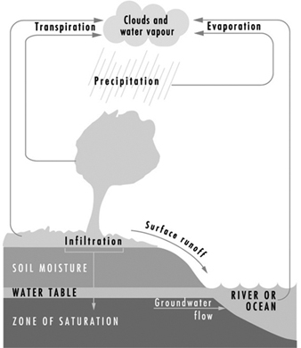
As a reference for water quality, distilled waters (H₂O) represent the highest state of purity. Waters in the hydrologic cycle may be viewed as natural, but are not pure. They become polluted from both natural and human activities. Natural degradation effects may result from a myriad of sources - from fauna, flora, volcano eruptions, lightning strikes causing fires and so on, which on a long-term basis are considered to be prevailing background levels for scientific purposes.

Human-made pollution disrupts the natural balance by superimposing waste materials discharged from various sources. Pollutants may be introduced into the waters of the hydrologic cycle at any point. For example: atmospheric precipitation (rainfall) may become contaminated by air pollutants; surface waters may become polluted in the runoff process from watersheds; sewage may be discharged into streams and rivers; and groundwaters may become polluted through infiltration and underground contamination.

Figure 2 shows a distribution of hydrologic waters. Pollution is then superimposed on these waters and may therefore be viewed as an unnatural or unbalanced environmental condition. The process of pollution may occur in waters of any part of the hydrologic cycle, and is more obvious on the earth’s surface in the form of runoff from watersheds into streams and rivers. However groundwater pollution is also of major environmental impact and is discussed following the section on surface water pollution.

Figure 2. Distribution of precipitation

Watershed sources of water pollution

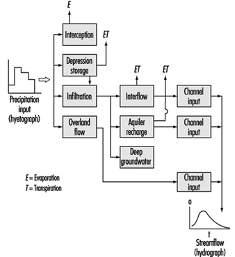
Watersheds are the originating domain of surface water pollution. A watershed is defined as an area of the earth’s surface on which hydrologic waters fall, accumulate, are used, disposed of, and eventually are discharged into streams, rivers or other bodies of water. It is comprised of a drainage system with ultimate runoff or collection in a stream or river. Large river watersheds are usually referred to as drainage basins. Figure 3 is a representation of the hydrologic cycle on a regional watershed. For a region, the disposition of the various waters can be written as a simple equation, which is the basic equation of hydrology as written by Viessman, Lewis and Knapp (1989); typical units are mm/year:

P - R - G - E - T = ±S

where:

P = precipitation (i.e., rainfall, snowfall, hail)

R = runoff or watershed surface flow

G = groundwater

E = evaporation

T = transpiration

S = surface storage

Figure 3. Regional hydrologic cycle

Precipitation is viewed as the initiating form in the above hydrologic budget. The term runoff is synonymous with stream flow. Storage refers to reservoirs or detention systems which collect waters; for example, a human-made dam (barrage) on a river creates a reservoir for purposes of water storage. Groundwater collects as a storage system and may flow from one location to another; it may be influent or effluent in relation to surface streams. Evaporation is a water surface phenomenon, and transpiration is associated with transmission from biota.

Although watersheds may vary greatly in size, certain drainage systems for water pollution designation are classified as urban or non-urban (agricultural, rural, undeveloped) in character. Pollution occurring within these drainage systems originates from the following sources:

Point sources: waste discharges into a receiving water body at a specific location, at a point such as a sewer pipe or some type of concentrated system outlet.

Non-point (dispersed) sources: pollution entering a receiving water body from dispersed sources in the watershed; uncollected rainfall runoff water drainage into a stream is typical. Non-point sources are also sometimes referred to as “diffuse” waters; however, the term dispersed is seen as more descriptive.

Intermittent sources: from a point or source which discharges under certain circumstances, such as with overloaded conditions; combined sewer overflows during heavy rainfall runoff periods are typical.

Water pollutants in streams and rivers

When deleterious waste materials from the above sources are discharged into streams or other bodies of water, they become pollutants which have been classified and described in a previous section. Pollutants or contaminants which enter a body of water can be further divided into:

• degradable (non-conservative) pollutants: impurities which eventually decompose into harmless substances or which may be removed by treatment methods; that is, certain organic materials and chemicals, domestic sewage, heat, plant nutrients, most bacteria and viruses, certain sediments
• non-degradable (conservative) pollutants: impurities which persist in the water environment and do not reduce in concentration unless diluted or removed through treatment; that is, certain organic and inorganic chemicals, salts, colloidal suspensions
• hazardous waterborne pollutants: complex forms of deleterious wastes including toxic trace metals, certain inorganic and organic compounds
• radionuclide pollutants: materials which have been subjected to a radioactive source.

Water pollution control regulations

Broadly applicable water pollution control regulations are generally promulgated by national governmental agencies, with more detailed regulations by states, provinces, municipalities, water districts, conservation districts, sanitation commissions and others. At the national and state (or province) levels, environmental protection agencies (EPAs) and ministries of health are usually charged with this responsibility. In the discussion of regulations below, the format and certain portions follow the example of the water quality standards currently applicable for the US State of Ohio.

Water quality use designations

The ultimate goal in the control of water pollution would be zero discharge of pollutants to water bodies; however, complete achievement of this objective is usually not cost effective. The preferred approach is to set limitations on waste disposal discharges for the reasonable protection of human health and the environment. Although these standards may vary widely in different jurisdictions, use designations for specific bodies of water are commonly the basis, as briefly addressed below.

Water supplies include:

• public water supply: waters which with conventional treatment will be suitable for human consumption
• agricultural supply: waters suitable for irrigation and livestock watering without treatment
• industrial/commercial supply: waters suitable for industrial and commercial uses with or without treatment.

Recreational activities include:

• bathing waters: waters which during certain seasons are suitable for swimming as approved for water quality along with protective conditions and facilities
• primary contact: waters which during certain seasons are suitable for full body contact recreation such as swimming, canoeing and underwater diving with minimal threat to public health as a result of water quality
• secondary contact: waters which during certain seasons are suitable for partial body contact recreation such as, but not limited to, wading, with minimal threat to public health as a result of water quality.

Public water resources are categorized as water bodies which lie within park systems, wetland, wildlife areas, wild, scenic and recreational rivers and publicly owned lakes, and waters of exceptional recreational or ecological significance.

Aquatic life habitats

Typical designations will vary according to climates, but relate to conditions in water bodies for supporting and maintaining certain aquatic organisms, especially various species of fish. For example, use designations in a temperate climate as subdivided in regulations for the State of Ohio Environmental Protection Agency (EPA) are listed below without detailed descriptions:

• warmwater
• limited warmwater
• exceptional warmwater
• modified warmwater
• seasonal salmonid
• coldwater
• limited resource water.

Water pollution control criteria

Natural waters and wastewaters are characterized in terms of their physical, chemical and biological composition. The principal physical properties and the chemical and biological constituents of wastewater and their sources are a lengthy list, reported in a textbook by Metcalf and Eddy (1991). Analytical methods for these determinations are given in a widely used manual entitled Standard Methods for the Examination of Water and Waste Water by the American Public Health Association (1995).

Each designated water body should be controlled according to regulations which may be comprised of both basic and more detailed numerical criteria as briefly discussed below.

Basic freedom from pollution. To the extent practical and possible, all bodies of water should attain the basic criteria of the “Five Freedoms from Pollution”:

1. free from suspended solids or other substances that enter the waters as a result of human activity and that will settle to form putrid or otherwise objectionable sludge deposits, or that will adversely affect aquatic life
2. free from floating debris, oil, scum and other floating materials entering the waters as a result of human activity in amounts sufficient to be unsightly or cause degradation
3. free from materials entering the waters as a result of human activity, producing colour, odour or other conditions in such degree as to create a nuisance
4. free from substances entering the waters as a result of human activity, in concentrations that are toxic or harmful to human, animal or aquatic life and/or are rapidly lethal in the mixing zone
5. free from nutrients entering the waters as a result of human activity, in concentrations that create nuisance growths of aquatic weeds and algae.

Water quality criteria are numerical limitations and guidelines for the control of chemical, biological and toxic constituents in bodies of water.

With over 70,000-plus chemical compounds in use today it is impractical to specify the control of each. However, criteria for chemicals can be established on the basis of limitations as they first of all relate to three major classes of consumption and exposure:

Class 1: Chemical criteria for protection of human health are of first major concern and should be set according to recommendations from governmental health agencies, the WHO and recognized health research organizations.

Class 2: Chemical criteria for control of agricultural water supply should be based on recognized scientific studies and recommendations which will protect against adverse effects on crops and livestock as a result of crop irrigation and livestock watering.

Class 3: Chemical criteria for protection of aquatic life should be based on recognized scientific studies regarding the sensitivity of these species to specific chemicals and also as related to human consumption of fish and sea foods.

Wastewater effluent criteria relate to limitations on pollutant constituents present in wastewater effluents and are a further method of control. They may be set as related to the water use designations of bodies of water and as they relate to the above classes for chemical criteria.

Biological criteria are based on water body habitat conditions which are needed to support aquatic life.

Organic content of wastewaters and natural waters

The gross content of organic matter is most important in characterizing the pollutional strength of both wastewater and natural waters. Three laboratory tests are commonly used for this purpose:

Biochemical oxygen demand (BOD): five-day BOD (BOD5) is the most widely used parameter; this test measures the dissolved oxygen used by micro-organisms in the biochemical oxidation of organic matter over this period.

Chemical oxygen demand (COD): this test is to measure the organic matter in municipal and industrial wastes that contain compounds that are toxic to biological life; it is a measure of the oxygen equivalent of the organic matter that can be oxidized.

Total organic carbon (TOC): this test is especially applicable to small concentrations of organic matter in water; it is a measure of the organic matter that is oxidized to carbon dioxide.

Antidegradation policy regulations

Antidegradation policy regulations are a further approach for preventing the spread of water pollution beyond certain prevailing conditions. As an example, the Ohio Environmental Protection Agency Water Quality Standards antidegradation policy consists of three tiers of protection:

Tier 1: Existing uses must be maintained and protected. No further water quality degradation is allowed that would interfere with existing designated uses.

Tier 2: Next, water quality better than that needed to protect uses must be maintained unless it is shown that a lower water quality is necessary for important economic or social development, as determined by the EPA Director.

Tier 3: Finally, the quality of water resource waters must be maintained and protected. Their existing ambient water quality is not to be degraded by any substances determined to be toxic or to interfere with any designated use. Increased pollutant loads are allowed to be discharged into water bodies if they do not result in lowering existing water quality.

Water pollution discharge mixing zones and waste load allocation modelling

Mixing zones are areas in a body of water which allow for treated or untreated wastewater discharges to attain stabilized conditions, as illustrated in figure 4 for a flowing stream. The discharge is initially in a transitory state which becomes progressively diluted from the source concentration to the receiving water conditions. It is not to be considered as a treatment entity and may be delineated with specific restrictions.

Figure 4. Mixing zones

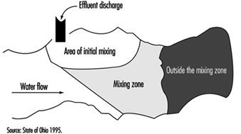
Typically, mixing zones must not:

• interfere with migration, survival, reproduction or growth of aquatic species

• include spawning or nursery areas

• include public water supply intakes

• include bathing areas

• constitute more than 1/2 the width of a stream

• constitute more than 1/2 the cross-sectional area of a stream mouth

• extend downstream for a distance more than five times the stream width.

Waste load allocation studies have become important because of the high cost of nutrient control of wastewater discharges to avoid instream eutrophication (defined below). These studies generally employ the use of computer models for simulation of water quality conditions in a stream, particularly with regard to nutrients such as forms of nitrogen and phosphorous, which affect the dissolved oxygen dynamics. Traditional water quality models of this type are represented by the US EPA model QUAL2E, which has been described by Brown and Barnwell (1987). A more recent model proposed by Taylor (1995) is the Omni Diurnal Model (ODM), which includes a simulation of the impact of rooted vegetation on instream nutrient and dissolved oxygen dynamics.

Variance provisions

All water pollution control regulations are limited in perfection and therefore should include provisions which allow for judgemental variance based on certain conditions which may prevent immediate or complete compliance.

Risk assessment and management as related to water pollution

The above water pollution control regulations are typical of worldwide governmental approaches for achieving compliance with water quality standards and wastewater effluent discharge limits. Generally these regulations have been set on the basis of health factors and scientific research; where some uncertainty exists as to possible effects, safety factors often are applied. Implementation of certain of these regulations may be unreasonable and exceedingly costly for the public at large as well as for private enterprise. Therefore there is a growing concern for more efficient allocation of resources in achieving goals for water quality improvement. As previously pointed out in the discussion of hydrologic waters, pristine purity does not exist even in naturally occurring waters.

A growing technological approach encourages assessment and management of ecological risks in the setting of water pollution regulations. The concept is based on an analysis of the ecological benefits and costs in meeting standards or limits. Parkhurst (1995) has proposed the application of aquatic ecological risk assessment as an aid in setting water pollution control limits, particularly as applicable for the protection of aquatic life. Such risk assessment methods may be applied to estimate the ecological effects of chemical concentrations for a broad range of surface water pollution conditions including:

• point source pollution

• non-point source pollution

• existing contaminated sediments in stream channels

• hazardous wastes sites as related to water bodies

• analysis of existing water pollution control criteria.

The proposed method consists of three tiers; as shown in figure 5 which illustrates the approach.

Figure 5. Methods for conducting risk assessment for successive tiers of analysis.  Tier 1: Screening level; Tier 2: Quantification of potentially significant risks ; Tier 3: Site-specific risk quantification

Water pollution in lakes and reservoirs

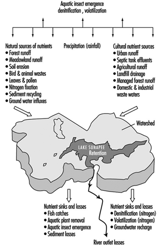
Lakes and reservoirs provide for the volumetric storage of watershed inflow and may have long flushing time periods as compared with the rapid inflow and outflow for a reach in a flowing stream. Therefore they are of special concern with regard to the retention of certain constituents, especially nutrients including forms of nitrogen and phosphorous which promote eutrophication. Eutrophication is a natural ageing process in which the water content becomes organically enriched, leading to the domination of undesirable aquatic growth, such as algae, water hyacinth and so on. The eutrophic process tends to decrease aquatic life and has detrimental dissolved oxygen effects. Both natural and cultural sources of nutrients may promote the process, as illustrated by Preul (1974) in figure 6, showing a schematic listing of nutrient sources and sinks for Lake Sunapee, in the US State of New Hampshire.

Figure 6. Schematic listing of nutrient (nitrogen and phosphorus) sources and sinks for  Lake Sunapee, New Hampshire (US)

Lakes and reservoirs, of course, can be sampled and analysed to determine their trophic status. Analytical studies usually start with a basic nutrient balance such as the following:

(lake influent nutrients) = (lake effluent nutrients) + (nutrient retention in lake)

This basic balance can be further expanded to include the various sources shown in figure 6.

Flushing time is an indication of the relative retention aspects of a lake system. Shallow lakes, such as Lake Erie, have relatively short flushing times and are associated with advanced eutrophication because shallow lakes often are more conducive to aquatic plant growth. Deep lakes such as Lake Tahoe and Lake Superior have very long flushing periods, which are usually associated with lakes with minimal eutrophication because up to the present time, they have not been overloaded and also because their extreme depths are not conducive to extensive aquatic plant growth except in the epilimnion (upper zone). Lakes in this category are generally classified as oligotrophic, on the basis that they are relatively low in nutrients and support minimal aquatic growth such as algae.

It is of interest to compare the flushing times of some major US lakes as reported by Pecor (1973) using the following calculation basis:

lake flushing time (LFT) = (lake storage volume)/(lake outflow)

Some examples are: Lake Wabesa (Michigan), LFT=0.30 years; Houghton Lake (Michigan), 1.4 years; Lake Erie, 2.6 years; Lake Superior, 191 years; Lake Tahoe, 700 years.

Although the relationship between the process of eutrophication and nutrient content is complex, phosphorous is typically recognized as the limiting nutrient. Based on fully mixed conditions, Sawyer (1947) reported that algal blooms tend to occur if nitrogen values exceed 0.3 mg/l and phosphorous exceeds 0.01 mg/l. In stratified lakes and reservoirs, low dissolved oxygen levels in the hypoliminion are early signs of eutrophication. Vollenweider (1968, 1969) has developed critical loading levels of total phosphorous and total nitrogen for a number of lakes based on nutrient loadings, mean depths and trophic states. For a comparison of work on this subject, Dillon (1974) has published a critical review of Vollenweider’s nutrient budget model and other related models. More recent computer models are also available for simulating nitrogen/phosphorous cycles with temperature variations.

Water pollution in estuaries

An estuary is an intermediate passageway of water between the mouth of a river and a sea coast. This passageway is comprised of a river mouth channel reach with river inflow (fresh water) from upstream and outflow discharge on the downstream side into a constantly changing tailwater level of sea water (salt water). Estuaries are continuously affected by tidal fluctuations and are among the most complex bodies of water encountered in water pollution control. The dominant features of an estuary are variable salinity, a salt wedge or interface between salt and fresh water, and often large areas of shallow, turbid water overlying mud flats and salt marshes. Nutrients are largely supplied to an estuary from the inflowing river and combine with the sea water habitat to provide prolific production of biota and sea life. Especially desired are seafoods harvested from estuaries.

From a water pollution standpoint, estuaries are individually complex and generally require special investigations employing extensive field studies and computer modelling. For a further basic understanding, the reader is referred to Reish 1979, on marine and estuarine pollution; and to Reid and Wood 1976, on the ecology of inland waters and estuaries.

Water pollution in marine environments

Oceans may be viewed as the ultimate receiving water or sink, since wastes carried by rivers finally discharge into this marine environment. Although oceans are vast bodies of salt water with seemingly unlimited assimilation capacity, pollution tends to blight coastlines and further affects marine life.

Sources of marine pollutants include many of those encountered in land-based wastewater environments plus more as related to marine operations. A limited list is given below:

• domestic sewage and sludge, industrial wastes, solid wastes, shipboard wastes

• fishery wastes, sediments and nutrients from rivers and land runoff

• oil spills, offshore oil exploration and production wastes, dredge operations

• heat, radioactive wastes, waste chemicals, pesticides and herbicides.

Each of the above requires special handling and methods of control. The discharge of domestic sewage and sewage sludges through ocean outfalls is perhaps the major source of marine pollution.

For current technology on this subject, the reader is referred to the book on marine pollution and its control by Bishop (1983).

Techniques for reducing pollution in wastewater discharges

Large-scale wastewater treatment is typically carried out by municipalities, sanitary districts, industries, commercial enterprises and various pollution control commissions. The purpose here is to describe contemporary methods of municipal wastewater treatment and then to provide some insights regarding treatment of industrial wastes and more advanced methods.

In general, all processes of wastewater treatment may be grouped into physical, chemical or biological types, and one or more of these may be employed to achieve a desired effluent product. This classification grouping is most appropriate in the understanding of wastewater treatment approaches and is tabulated in table 1.

Table 1. General classification of wastewater treatment operations and processes

Contemporary methods of wastewater treatment

The coverage here is limited and is intended to provide a conceptual overview of current wastewater treatment practices around the world rather than detailed design data. For the latter, the reader is referred to Metcalf and Eddy 1991.

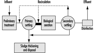
Municipal wastewaters along with some intermingling of industrial/commercial wastes are treated in systems commonly employing primary, secondary and tertiary treatment as follows:

Primary treatment system: Pre-treat ® Primary settling ® Disinfection (chlorination) ® Effluent

Secondary treatment system: Pre-treat ® Primary settling ® Biological unit ® Second settling ® Disinfection (chlorination) ® Effluent to stream

Tertiary treatment system: Pre-treat ® Primary settling ® Biological unit ® Second settling ® Tertiary unit ® Disinfection (chlorination) ® Effluent to stream

Figure 7 further shows a schematic diagram of a conventional wastewater treatment system. Overview descriptions of the above processes follow.

Figure 7. Schematic diagram of conventional wastewater treatment

Primary treatment

The basic objective of primary treatment for municipal wastewaters, including domestic sewage intermingled with some industrial/commercial wastes, is to remove suspended solids and clarify the wastewater, to make it suitable for biological treatment. After some pre-treatment handling such as screening, grit removal and comminution, the main process of primary sedimentation is the settling of the raw wastewater in large settling tanks for periods up to several hours. This process removes from 50 to 75% of the total suspended solids, which are drawn off as an underflow sludge collected for separate treatment. The overflow effluent from the process then is directed for secondary treatment. In certain cases, chemicals may be employed to improve the degree of primary treatment.

Secondary treatment

The portion of the organic content of the wastewater which is finely suspended or dissolved and not removed in the primary process, is treated by secondary treatment. The generally accepted forms of secondary treatment in common use include trickling filters, biological contactors such as rotating discs, activated sludge, waste stabilization ponds, aerated pond systems and land application methods, including wetland systems. All of these systems will be recognized as employing biological processes of some form or another. The most common of these processes are briefly discussed below.

Biological contactor systems. Trickling filters are one of the earliest forms of this method for secondary treatment and are still widely used with some improved methods of application. In this treatment, the effluent from the primary tanks is applied uniformly onto a bed of media, such as rock or synthetic plastic media. Uniform distribution is accomplished typically by trickling the liquid from perforated piping rotated over the bed intermittently or continuously according to the desired process. Depending on the rate of organic and hydraulic loadings, trickling filters can remove up to 95% of the organic content, usually analysed as biochemical oxygen demand (BOD). There are numerous other more recent biological contactor systems in use which can provide treatment removals in the same range; some of these methods offer special advantages, particularly applicable in certain limiting conditions such as space, climate and so on. It is to be noted that a following secondary settling tank is considered to be a necessary part of completing the process. In secondary settling, some so-called humus sludge is drawn off as an underflow, and the overflow is discharged as a secondary effluent.

Activated sludge. In the most common form of this biological process, primary treated effluent flows into an activated sludge unit tank containing a previously existing biological suspension called activated sludge. This mixture is referred to as mixed liquor suspended solids (MLSS) and is provided a contact period typically ranging from several hours up to 24 hours or more, depending on the desired results. During this period the mixture is highly aerated and agitated to promote aerobic biological activity. As the process finalizes, a portion of the mixture (MLSS) is drawn off and returned to the influent for continuation of the biological activation process. Secondary settling is provided following the activated sludge unit for the purpose of settling out the activated sludge suspension and discharging a clarified overflow as an effluent. The process is capable of removing up to about 95% of the influent BOD.

Tertiary treatment

A third level of treatment may be provided where a higher degree of pollutant removal is required. This form of treatment may typically include sand filtration, stabilization ponds, land disposal methods, wetlands and other systems which further stabilize the secondary effluent.

Disinfection of effluents

Disinfection is commonly required to reduce bacteria and pathogens to acceptable levels. Chlorination, chlorine dioxide, ozone and ultraviolet light are the most commonly used processes.

Overall wastewater treatment plant efficiency

Wastewaters include a broad range of constituents which generally are classified as suspended and dissolved solids, inorganic constituents and organic constituents.

The efficiency of a treatment system can be measured in terms of the percentage removal of these constituents. Common parameters of measurement are:

• BOD: biochemical oxygen demand, measured in mg/l

• COD: chemical oxygen demand, measured in mg/l

• TSS: total suspended solids, measured in mg/l

• TDS: total dissolved solids, measured in mg/l

• nitrogen forms: including nitrate and ammonia, measured in mg/l (nitrate is of particular concern as a nutrient in eutrophication)

• phosphate: measured in mg/l (also of particular concern as a nutrient in eutrophication)

• pH: degree of acidity, measured as a number from 1 (most acid) to 14 (most alkaline)

• coliform bacteria counts: measured as most probable number per 100 ml (Escherichia and fecal coliform bacteria are most common indicators).

Industrial wastewater treatment

Types of industrial wastes

Industrial (non-domestic) wastes are numerous and vary greatly in composition; they may be highly acidic or alkaline, and often require a detailed laboratory analysis. Specialized treatment may be necessary to render them innocuous before discharge. Toxicity is of great concern in the disposal of industrial wastewaters.

Representative industrial wastes include: pulp and paper, slaughterhouse, brewery, tannery, food processing, cannery, chemical, petroleum, textile, sugar, laundry, meat and poultry, hog feeding, rendering and many others. The initial step in treatment design development is an industrial waste survey, which provides data on variations in flow and waste characteristics. Undesirable waste characteristics as listed by Eckenfelder (1989) can be summarized as follows:

• soluble organics causing depletion of dissolved oxygen

• suspended solids

• trace organics

• heavy metals, cyanide and toxic organics

• colour and turbidity

• nitrogen and phosphorus

• refractory substances resistant to biodegradation

• oil and floating material

• volatile materials.

The US EPA has further defined a list of toxic organic and inorganic chemicals with specific limitations in granting discharge permits. The list includes more than 100 compounds and is too long to reprint here, but may be requested from the EPA.

Treatment methods

The handling of industrial wastes is more specialized than the treatment of domestic wastes; however, where amenable to biological reduction, they are usually treated using methods similar to those previously described (secondary/tertiary biological treatment approaches) for municipal systems.

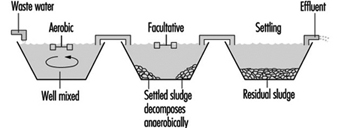
Waste stabilization ponds are a common method of organic wastewater treatment where sufficient land area is available. Flow-through ponds are generally classified according to their bacterial activity as aerobic, facultative or anaerobic. Aerated ponds are supplied with oxygen by diffused or mechanical aeration systems.

Figure 8 and figure 9 show sketches of waste stabilization ponds.

Figure 8.  Two-cell stabilization pond: cross sectional diagram

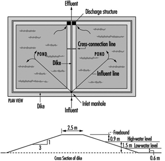
Figure 9. Aerated lagoon types: schematic diagram

Pollution prevention and waste minimization

When industrial waste in-plant operations and processes are analysed at their source, they often can be controlled so as to prevent significant polluting discharges.

Recirculation techniques are important approaches in pollution prevention programmes. A case study example is a recycling plan for a leather tannery wastewater effluent published by Preul (1981), which included chrome recovery/reuse along with the complete recirculation of all tannery wastewaters with no effluent to any stream except in emergencies. The flow diagram for this system is shown in figure 10.

Figure 10. Flow diagram for tannery wastewater effluent recycling system

For more recent innovations in this technology, the reader is referred to a publication on pollution prevention and waste minimization by the Water Environment Federation (1995).

Advanced methods of wastewater treatment

A number of advanced methods are available for higher degrees of removal of pollution constituents as may be required. A general listing includes:

filtration (sand and multimedia)

chemical precipitation

carbon adsorption

electrodialysis

distillation

nitrification

algae harvesting

reclamation of effluents

micro-straining

ammonia stripping

reverse osmosis

ion exchange

land application

denitrification

wetlands.

The most appropriate process for any situation must be determined on the basis of the quality and quantity of the raw wastewater, the receiving water requirements and, of course, costs. For further reference, see Metcalf and Eddy 1991, which includes a chapter on advanced wastewater treatment.

Advanced wastewater treatment case study

The case study of the Dan Region Sewage Reclamation Project discussed elsewhere in this chapter provides an excellent example of innovative methods for wastewater treatment and reclamation.

Thermal pollution

Thermal pollution is a form of industrial waste, defined as deleterious increases or reductions in normal water temperatures of receiving waters caused by the disposal of heat from human-made facilities. The industries producing major waste heat are fossil fuel (oil, gas and coal) and nuclear power generating plants, steel mills, petroleum refineries, chemical plants, pulp and paper mills, distilleries and laundries. Of particular concern is the electric power generating industry which supplies energy for many countries (e.g., about 80% in the US).

Impact of waste heat on receiving waters

Influence on waste assimilation capacity

• Heat increases biological oxidation.

• Heat decreases oxygen saturation content of water and decreases rate of natural reoxygenation.

• The net effect of heat is generally detrimental during warm months of year.

• Winter effect may be beneficial in colder climates, where ice conditions are broken up and surface aeration is provided for fish and aquatic life.

Influence on aquatic life

Many species have temperature tolerance limits and need protection, particularly in heat affected reaches of a stream or body of water. For example, cold water streams usually have the highest type of sport fish such as trout and salmon, whereas warm waters generally support coarse fish populations, with certain species such as pike and bass fish in intermediate temperature waters.

Figure 11. Heat exchange at the boundaries of a receiving water cross section

Thermal analysis in receiving waters

Figure 11 illustrates the various forms of natural heat exchange at the boundaries of a receiving water. When heat is discharged to a receiving water such as a river, it is important to analyse the river capacity for thermal additions. The temperature profile of a river can be calculated by solving a heat balance similar to that used in calculating dissolved oxygen sag curves. The principal factors of the heat balance are illustrated in figure 12 for a river reach between points A and B. Each factor requires an individual calculation dependent on certain heat variables. As with a dissolved oxygen balance, the temperature balance is simply a summation of temperature assets and liabilities for a given section. Other more sophisticated analytical approaches are available in the literature on this subject. The results from the heat balance calculations can be used in establishing heat discharge limitations and possibly certain use constraints for a body of water.

Figure 12. River capacity for thermal additions

Thermal pollution control

The main approaches for the control of thermal pollution are:

• improved power plant operation efficiencies

• cooling towers

• isolated cooling ponds

• consideration of alternative methods of power generation such as hydro-power.

Where physical conditions are favourable within certain environmental limits, hydro-electric power should be considered as an alternative to fossil-fuel or nuclear power generation. In hydro-electric power generation, there is no disposal of heat and there is no discharge of waste waters causing water pollution.

Groundwater Pollution Control

Importance of groundwater

Since the world’s water supplies are widely extracted from aquifers, it is most important that these sources of supply be protected. It is estimated that more than 95% of the earth’s available fresh water supply is underground; in the United States approximately 50% of the drinking water comes from wells, according to the 1984 US Geological Survey. Because underground water pollution and movement are of subtle and unseen nature, less attention sometimes is given to the analysis and control of this form of water degradation than to surface water pollution, which is far more obvious.

Figure 13.  Hydrologic cycle and sources of groundwater contamination

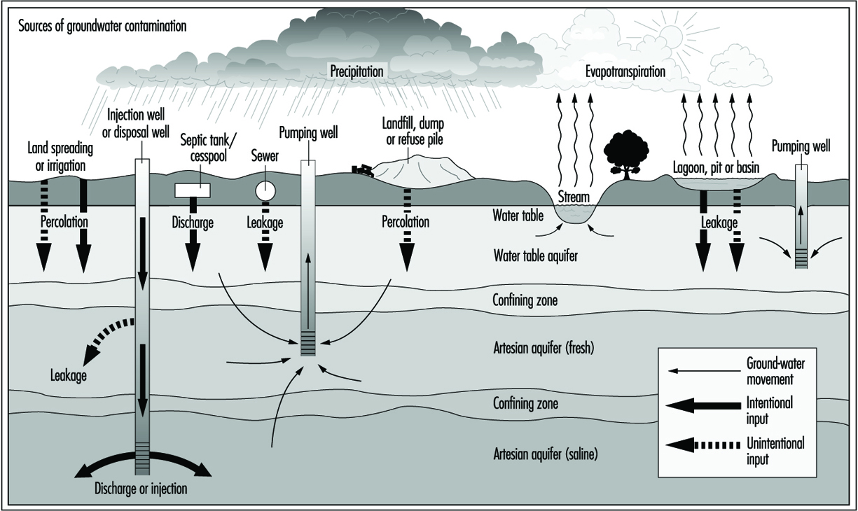
Sources of underground pollution

Figure 13 shows the hydrologic cycle with superimposed sources of groundwater contamination. A complete listing of the potential sources of underground pollution is extensive; however, for illustration the most obvious sources include:

• industrial waste discharges

• polluted streams in contact with aquifers

• mining operations

• solid and hazardous waste disposal

• underground storage tanks such as for petroleum

• irrigation systems

• artificial recharge

• sea water encroachment

• spills

• polluted ponds with permeable bottoms

• disposal wells

• septic tank tile fields and leaching pits

• improper well drilling

• agricultural operations

• roadway de-icing salts.

Specific pollutants in underground contamination are further categorized as:

• undesirable chemical constituents (typical, not complete list) - organic and inorganic (e.g., chloride, sulphate, iron, manganese, sodium, potassium)

• total hardness and total dissolved solids

• toxic constituents (typical, not complete list) - nitrate, arsenic, chromium, lead, cyanide, copper, phenols, dissolved mercury

• undesirable physical characteristics - taste, colour and odour

• pesticides and herbicides - chlorinated hydrocarbons and others

• radioactive materials - various forms of radioactivity

• biological - bacteria, viruses, parasites and so on

• acid (low pH) or caustic (high pH).

Of the above, nitrates are of special concern in both ground waters and surface waters. In groundwater supplies, nitrates can cause the disease methaemoglobinaemia (infant cyanosis). They further cause detrimental eutrophication effects in surface waters and occur in a wide range of water resources, as reported by Preul (1991). Preul (1964, 1967, 1972) and Preul and Schroepfer (1968) have also reported on the underground movement of nitrogen and other pollutants.

Pollution travel in underground domain

Groundwater movement is exceedingly slow and subtle as compared with the travel of surface waters in the hydrologic cycle. For a simple understanding of the travel of ordinary groundwater under ideal steady flow conditions, Darcy’s Law is the basic approach for the evaluation of groundwater movement at low Reynolds numbers (R):

V = K(dh/dl)

where:

V = velocity of groundwater in aquifer, m/day

K = coefficient of permeability of aquifer

(dh/dl) = hydraulic gradient which represents the driving force for movement.

In pollutant travel underground, ordinary groundwater (H₂O) is generally the carrying fluid and can be calculated to move at a rate according to the parameters in Darcy’s Law. However, the rate of travel or velocity of a pollutant, such as an organic or inorganic chemical, may be different due to advection and hydrodynamic dispersion processes. Certain ions move slower or faster than the general rate of groundwater flow as a result of reactions within the aquifer media, so that they can be categorized as “reacting” or “non-reacting”. Reactions are generally of the following forms:

• physical reactions between the pollutant and the aquifer and/or the transporting liquid

• chemical reactions between the pollutant and the aquifer and/or the transporting liquid

• biological actions on the pollutant.

The following are typical of reacting and non-reacting underground pollutants:

• reacting pollutants - chromium, ammonium ion, calcium, sodium, iron and so on; cations in general; biological constituents; radioactive constituents

• non-reacting pollutants - chloride, nitrate, sulphate and so on; certain anions; certain pesticide and herbicide chemicals.

At first, it might seem that reacting pollutants are the worst type, but this may not always be the case because the reactions detain or retard pollutant travel concentrations whereas non-reacting pollutant travel may be largely uninhibited. Certain “soft” domestic and agricultural products are now available which biologically degrade after a period of time and therefore avoid the possibility of groundwater contamination.

Aquifer remediation

Prevention of underground pollution is obviously the best approach; however, uncontrolled existence of polluted groundwater conditions usually is made known after its occurrence, such as by complaints from water well users in the area. Unfortunately, by the time the problem is recognized, severe damage may have occurred and remediation is necessary. Remediation may require extensive hydro-geological field investigations with laboratory analyses of water samples in order to establish the extent of pollutant concentrations and travel plumes. Often existing wells can be used in initial sampling, but severe cases may require extensive borings and water samplings. These data can then be analysed to establish current conditions and to make future condition predictions. The analysis of groundwater contamination travel is a specialized field often requiring the use of computer models to better understand the groundwater dynamics and to make predictions under various constraints. A number of two- and three-dimensional computer models are available in the literature for this purpose. For more detailed analytical approaches, the reader is referred to the book by Freeze and Cherry (1987).

Pollution prevention

The preferred approach for the protection of groundwater resources is pollution prevention. Although drinking water standards generally apply to the use of groundwater supplies, the raw water supplies require protection from contamination. Governmental entities such as ministries of health, natural resources agencies, and environmental protection agencies are generally responsible for such activities. Groundwater pollution control efforts are largely directed at protection of aquifers and the prevention of pollution.

Pollution prevention requires land-use controls in the form of zoning and certain regulations. Laws may apply to the prevention of specific functions as particularly applicable to point sources or actions which potentially may cause pollution. Control by land-use zoning is a groundwater protection tool which is most effective at the municipal or county level of government. Aquifer and wellhead protection programmes as discussed below are leading examples of pollution prevention.

An aquifer protection programme requires establishing the boundaries of the aquifer and its recharge areas. Aquifers may be of an unconfined or confined type, and therefore need to be analysed by a hydrologist to make this determination. Most major aquifers are generally well known in developed countries, but other areas may require field investigations and hydrogeologic analysis. The key element of the programme in the protection of the aquifer from water quality degradation is control of land use over the aquifer and its recharge areas.

Wellhead protection is a more definitive and limited approach which applies to the recharge area contributing to a particular well. The US federal government by amendments passed in 1986 to the Safe Drinking Water Act (SDWA) (1984) now requires that specific wellhead protection areas be established for public supply wells. The wellhead protection area (WHPA) is defined in the SDWA as “the surface and subsurface area surrounding a water well or well field, supplying a public water supply system, through which contaminants are reasonably likely to move toward and reach such water well or well field.” The main objective in the WHPA programme, as outlined by the US EPA (1987), is the delineation of well protection areas based on selected criteria, well operation and hydrogeologic considerations.

Back

Management of Air Pollution

The objective of a manager of an air pollution control system is to ensure that excessive concentrations of air pollutants do not reach a susceptible target. Targets could include people, plants, animals and materials. In all cases we should be concerned with the most sensitive of each of these groups. Air pollutants could include gases, vapours, aerosols and, in some cases, biohazardous materials. A well designed system will prevent a target from receiving a harmful concentration of a pollutant.

Most air pollution control systems involve a combination of several control techniques, usually a combination of technological controls and administrative controls, and in larger or more complex sources there may be more than one type of technological control.

Ideally, the selection of the appropriate controls will be made in the context of the problem to be solved.

• What is emitted, in what concentration?
• What are the targets? What is the most susceptible target?
• What are acceptable short-term exposure levels?
• What are acceptable long-term exposure levels?
• What combination of controls must be selected to ensure that the short-term and long-term exposure levels are not exceeded?

Table 1 describes the steps in this process.

Table 1. Steps in selecting pollution controls

* When setting exposure levels in Step 3, it must be remembered that these exposures are total exposures, not just those from the plant. Once the acceptable level has been established, background levels, and contributions from other plants just be subtracted to determine the maximum amount that the plant can emit without exceeding the acceptable exposure level. If this is not done, and three plants are allowed to emit at the maximum amount, the target groups will be exposed to three times the acceptable level.

** Some materials such as carcinogens do not have a threshold below which no harmful effects will occur. Therefore, as long as some of the material is allowed to escape to the environment, there will be some risk to the target populations. In this case a no effect level cannot be set (other than zero). Instead, an acceptable level of risk must be established. Usually this is set in the range of 1 adverse outcome in 100,000 to 1,000,000 exposed persons.

Some jurisdictions have done some of the work by setting standards based on the maximum concentration of a contaminant that a susceptible target can receive. With this type of standard, the manager does not have to carry out Steps 2 and 3, since the regulating agency has already done this. Under this system, the manager must establish only the uncontrolled emission standards for each pollutant (Step 1), and then determine what controls are necessary to meet the standard (Step 4).

By having air quality standards, regulators can measure individual exposures and thus determine whether anyone is exposed to potentially harmful levels. It is assumed that the standards set under these conditions are low enough to protect the most susceptible target group. This is not always a safe assumption. As shown in table 2, there can be a wide variation in common air quality standards. Air quality standards for sulphur dioxide range from 30 to 140 μg/m³. For less commonly regulated materials this variation can be even larger (1.2 to 1,718 μg/m³), as shown in table 3 for benzene. This is not surprising given that economics can play as large a role in standard setting as does toxicology. If a standard is not set low enough to protect susceptible populations, no one is well served. Exposed populations have a feeling of false confidence, and can unknowingly be put at risk. The emitter may at first feel that they have benefited from a lenient standard, but if effects in the community require the company to redesign their controls, or install new controls, costs could be higher than doing it correctly the first time.

Table 2. Range of air quality standards for a commonly controlled air contaminant (sulphur dioxide)

Table 3. Range of air quality standards for a less commonly controlled air contaminant (benzene)

The levels were standardized to an averaging time of 24 hours to assist in the comparisons.

(Adapted from Calabrese and Kenyon 1991.)

Sometimes this stepwise approach to selecting air pollution controls is short circuited, and the regulators and designers go directly to a “universal solution”. One such method is best available control technology (BACT). It is assumed that by using the best combination of scrubbers, filters and good work practices on an emission source, a level of emissions low enough to protect the most susceptible target group would be achieved. Frequently, the resulting emission level will be below the minimum required to protect the most susceptible targets. This way all unnecessary exposures should be eliminated. Examples of BACT are shown in table 4.

Table 4. Selected examples of best available control technology (BACT) showing the control method used and estimated efficiency

BACT by itself does not ensure adequate control levels. Although this is the best control system based on gas cleaning controls and good operating practices, BACT may not be good enough if the source is a large plant, or if it is located next to a sensitive target. Best available control technology should be tested to ensure that it is indeed good enough. The resulting emission standards should be checked to determine whether or not they may still be harmful even with the best gas cleaning controls. If emission standards are still harmful, other basic controls, such as selecting safer processes or materials, or relocating in a less sensitive area, may have to be considered.

Another “universal solution” that bypasses some of the steps is source performance standards. Many jurisdictions establish emission standards that cannot be exceeded. Emission standards are based on emissions at the source. Usually this works well, but like BACT they can be unreliable. The levels should be low enough to maintain the maximum emissions low enough to protect susceptible target populations from typical emissions. However, as with best available control technology, this may not be good enough to protect everyone where there are large emission sources or nearby susceptible populations. If this is the case, other procedures must be used to ensure the safety of all target groups.

Both BACT and emission standards have a basic fault. They assume that if certain criteria are met at the plant, the target groups will be automatically protected. This is not necessarily so, but once such a system is passed into law, effects on the target become secondary to compliance with the law.

BACT and source emission standards or design criteria should be used as minimum criteria for controls. If BACT or emission criteria will protect the susceptible targets, then they can be used as intended, otherwise other administrative controls must be used.

Control Measures

Controls can be divided into two basic types of controls - technological and administrative. Technological controls are defined here as the hardware put on an emission source to reduce contaminants in the gas stream to a level that is acceptable to the community and that will protect the most sensitive target. Administrative controls are defined here as other control measures.

Technological controls

Gas cleaning systems are placed at the source, before the stack, to remove contaminants from the gas stream before releasing it to the environment. Table 5 shows a brief summary of the different classes of gas cleaning system.

Table 5. Gas cleaning methods for removing harmful gases, vapours and particulates from industrial process emissions

The gas cleaner is part of a complex system consisting of hoods, ductwork, fans, cleaners and stacks. The design, performance and maintenance of each part affects the performance of all other parts, and the system as a whole.

It should be noted that system efficiency varies widely for each type of cleaner, depending on its design, energy input and the characteristics of the gas stream and the contaminant. As a result, the sample efficiencies in table 5 are only approximations. The variation in efficiencies is demonstrated with wet scrubbers in table 5. Wet scrubber collection efficiency goes from 98.5 per cent for 5 μm particles to 45 per cent for 1 μm particles at the same pressure drop across the scrubber (6.8 in. water gauge (w.g.)). For the same size particle, 1 μm, efficiency goes from 45 per cent efficiency at 6.8 w.g. to 99.95 at 50 w.g. As a result, gas cleaners must be matched to the specific gas stream in question. The use of generic devices is not recommended.

Waste disposal

When selecting and designing gas cleaning systems, careful consideration must be given to the safe disposal of the collected material. As shown in table 6, some processes produce large amounts of contaminants. If most of the contaminants are collected by the gas cleaning equipment there can be a hazardous waste disposal problem.

Table 6. Sample uncontrolled emission rates for selected industrial processes

In some cases the wastes may contain valuable products that can be recycled, such as heavy metals from a smelter, or solvent from a painting line. The wastes can be used as a raw material for another industrial process - for example, sulphur dioxide collected as sulphuric acid can be used in the manufacture of fertilizers.

Where the wastes cannot be recycled or reused, disposal may not be simple. Not only can the volume be a problem, but they may be hazardous themselves. For example, if the sulphuric acid captured from a boiler or smelter cannot be reused, it will have to be further treated to neutralize it before disposal.

Dispersion

Dispersion can reduce the concentration of a pollutant at a target. However, it must be remembered that dispersion does not reduce the total amount of material leaving a plant. A tall stack only allows the plume to spread out and be diluted before it reaches ground level, where susceptible targets are likely to exist. If the pollutant is primarily a nuisance, such as an odour, dispersion may be acceptable. However if the material is persistent or cumulative, such as heavy metals, dilution may not be an answer to an air pollution problem.

Dispersion should be used with caution. Local meteorological and ground surface conditions must be taken into consideration. For example, in colder climates, particularly with snow cover, there can be frequent temperature inversions that can trap pollutants close to the ground, resulting in unexpectedly high exposures. Similarly, if a plant is located in a valley, the plumes may move up and down the valley, or be blocked by surrounding hills so that they do not spread out and disperse as expected.

Administrative controls

In addition to the technological systems, there is another group of controls that must be considered in the overall design of an air pollution control system. For the large part, they come from the basic tools of industrial hygiene.

Substitution

One of the preferred occupational hygiene methods for controlling environmental hazards in the workplace is to substitute a safer material or process. If a safer process or material can be used, and harmful emissions avoided, the type or efficacy of controls becomes academic. It is better to avoid the problem than it is to try to correct a bad first decision. Examples of substitution include the use of cleaner fuels, covers for bulk storage and reduced temperatures in dryers.

This applies to minor purchases as well as the major design criteria for the plant. If only environmentally safe products or processes are purchased, there will be no risk to the environment, indoors or out. If the wrong purchase is made, the remainder of the programme consists of trying to compensate for that first decision. If a low-cost but hazardous product or process is purchased it may need special handling procedures and equipment, and special disposal methods. As a result, the low-cost item may have only a low purchase price, but a high price to use and dispose of it. Perhaps a safer but more expensive material or process would have been less costly in the long run.

Local ventilation

Controls are required for all the identified problems that cannot be avoided by substituting safer materials or methods. Emissions start at the individual worksite, not the stack. A ventilation system that captures and controls emissions at the source will help protect the community if it is properly designed. The hoods and ducts of the ventilation system are part of the total air pollution control system.

A local ventilation system is preferred. It does not dilute the contaminants, and provides a concentrated gas stream that is easier to clean before release to the environment. Gas cleaning equipment is more efficient when cleaning air with higher concentrations of contaminants. For example, a capture hood over the pouring spout of a metal furnace will prevent contaminants from getting into the environment, and deliver the fumes to the gas cleaning system. In table 5 it can be seen that cleaning efficiencies for absorption and adsorption cleaners increase with the concentration of the contaminant, and condensation cleaners are not recommended for low levels (<2,000 ppm) of contaminants.

If pollutants are not caught at the source and are allowed to escape through windows and ventilation openings, they become uncontrolled fugitive emissions. In some cases, these uncontrolled fugitive emissions can have a significant impact on the immediate neighbourhood.

Isolation

Isolation - locating the plant away from susceptible targets - can be a major control method when engineering controls are inadequate by themselves. This may be the only means of achieving an acceptable level of control when best available control technology (BACT) must be relied on. If, after applying the best available controls, a target group is still at risk, consideration must be given to finding an alternate site where sensitive populations are not present.

Isolation, as presented above, is a means of separating an individual plant from susceptible targets. Another isolation system is where local authorities use zoning to separate classes of industries from susceptible targets. Once industries have been separated from target populations, the population should not be allowed to relocate next to the facility. Although this seems like common sense, it isn’t employed as often as it should be.

Work procedures

Work procedures must be developed to ensure that equipment is used properly and safely, without risk to workers or the environment. Complex air pollution systems must be properly maintained and operated if they are to do their job as intended. An important factor in this is staff training. Staff must be trained in how to use and maintain the equipment to reduce or eliminate the amount of hazardous materials emitted to the workplace or the community. In some cases BACT relies on good practice to ensure acceptable results.

Real time monitoring

A system based on real time monitoring is not popular, and is not commonly used. In this case, continuous emission and meteorological monitoring can be combined with dispersion modelling to predict downwind exposures. When the predicted exposures approach the acceptable levels, the information is used to reduce production rates and emissions. This is an inefficient method, but may be an acceptable interim control method for an existing facility.

The converse of this to announce warnings to the public when conditions are such that excessive concentrations of contaminants may exist, so that the public can take appropriate action. For example, if a warning is sent out that atmospheric conditions are such that sulphur dioxide levels downwind of a smelter are excessive, susceptible populations such as asthmatics would know not to go outside. Again, this may be an acceptable interim control until permanent controls are installed.

Real time atmospheric and meteorological monitoring is sometimes used to avoid or reduce major air pollution events where multiple sources may exist. When it becomes evident that excessive air pollution levels are likely, the personal use of cars may be restricted and major emitting industries shut down.

Maintenance/housekeeping

In all cases the effectiveness of the controls depends on proper maintenance; the equipment has to operate as intended. Not only must the air pollution controls be maintained and used as intended, but the processes generating potential emissions must be maintained and operated properly. An example of an industrial process is a wood chip dryer with a failing temperature controller; if the dryer is operated at too high a temperature, it will emit more materials, and perhaps a different type of material, from the drying wood. An example of gas cleaner maintenance affecting emissions would be a poorly maintained baghouse with broken bags, which would allow particulates to pass through the filter.

Housekeeping also plays an important part in controlling total emissions. Dusts that are not quickly cleaned up inside the plant can become re-entrained and present a hazard to staff. If the dusts are carried outside of the plant, they are a community hazard. Poor housekeeping in the plant yard could present a significant risk to the community. Uncovered bulk materials, plant wastes or vehicle-raised dusts can result in pollutants being carried on the winds into the community. Keeping the yard clean, using proper containers or storage sites, is important in reducing total emissions. A system must be not only designed properly, but used properly as well if the community is to be protected.

A worst case example of poor maintenance and housekeeping would be the lead recovery plant with a broken lead dust conveyor. The dust was allowed to escape from the conveyor until the pile was so high the dust could slide down the pile and out a broken window. Local winds then carried the dust around the neighbourhood.

Equipment for Emission Sampling

Source sampling can be carried out for several reasons:

• To characterize the emissions. To design an air pollution control system, one must know what is being emitted. Not only the volume of gas, but the amount, identity and, in the case of particulates, size distribution of the material being emitted must be known. The same information is necessary to catalogue total emissions in a neighbourhood.

• To test equipment efficiency. After an air pollution control system has been purchased, it should be tested to ensure that it is doing the intended job.

• As part of a control system. When emissions are continuously monitored, the data can be used to fine tune the air pollution control system, or the plant operation itself.

• To determine compliance. When regulatory standards include emission limits, emission sampling can be used to determine compliance or non-compliance with the standards.

The type of sampling system used will depend on the reason for taking the samples, costs, availability of technology, and training of staff.

Visible emissions

Where there is a desire to reduce the soiling power of the air, improve visibility or prevent the introduction of aerosols into the atmosphere, standards may be based on visible emissions.

Visible emissions are composed of small particles or coloured gases. The more opaque a plume is, the more material is being emitted. This characteristic is evident to the sight, and trained observers can be used to assess emission levels. There are several advantages to using this method of assessing emission standards:

• No expensive equipment is required.

• One person can make many observations in a day.

• Plant operators can quickly assess the effects of process changes at low cost.

• Violators can be cited without time-consuming source testing.

• Questionable emissions can be located and the actual emissions then determined by source testing as described in the following sections.

Extractive sampling

A much more rigorous sampling method calls for a sample of the gas stream to be removed from the stack and analysed. Although this sounds simple, it does not translate into a simple sampling method.

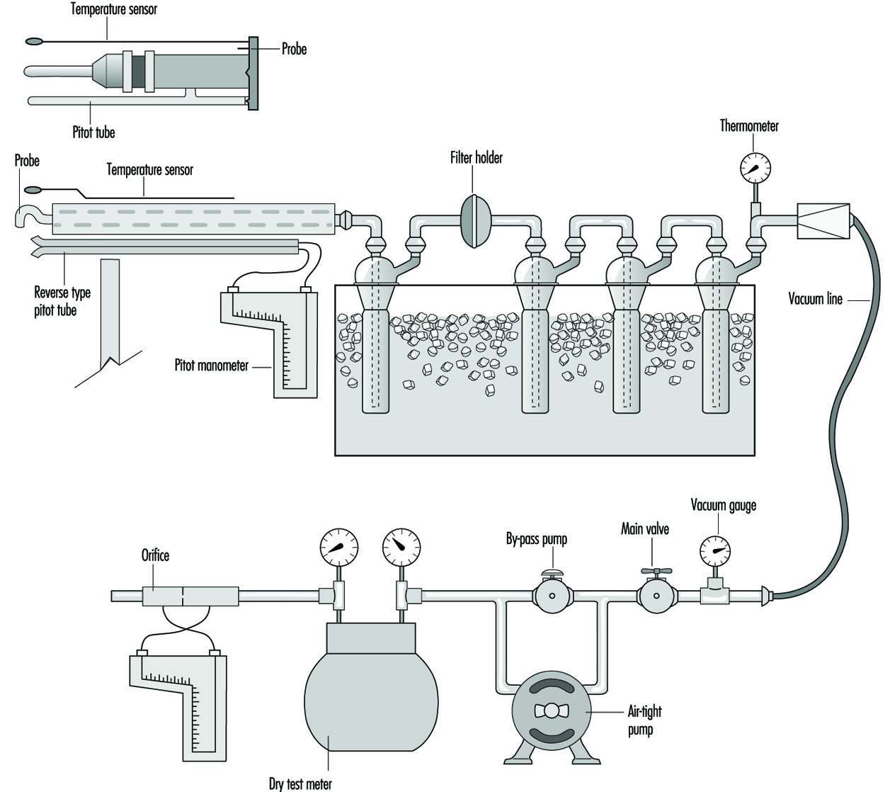
The sample should be collected isokinetically, especially when particulates are being collected. Isokinetic sampling is defined as sampling by drawing the sample into the sampling probe at the same velocity that the material is moving in the stack or duct. This is done by measuring the velocity of the gas stream with a pitot tube and then adjusting the sampling rate so that the sample enters the probe at the same velocity. This is essential when sampling for particulates, since larger, heavier particles will not follow a change in direction or velocity. As a result the concentration of larger particles in the sample will not be representative of the gas stream and the sample will be inaccurate.

A sample train for sulphur dioxide is shown in figure 1. It is not simple, and a trained operator is required to ensure that a sample is collected properly. If something other than sulphur dioxide is to be sampled, the impingers and ice bath can be removed and the appropriate collection device inserted.

Figure 1. A diagram of an isokinetic sampling train for sulphur dioxide

Extractive sampling, particularly isokinetic sampling, can be very accurate and versatile, and has several uses:

• It is a recognized sampling method with adequate quality controls, and thus can be used to determine compliance with standards.

• The potential accuracy of the method makes it suitable for performance testing of new control equipment.

• Since samples can be collected and analysed under controlled laboratory conditions for many components, it is useful for characterizing the gas stream.

A simplified and automated sampling system can be connected to a continuous gas (electrochemical, ultraviolet-photometric or flame ionization sensors) or particulate (nephelometer) analyzer to continuously monitor emissions. This can provide documentation of the emissions, and instantaneous operating status of the air pollution control system.

In situ sampling

Emissions can also be sampled in the stack. Figure 2 is a representation of a simple transmissometer used to measure materials in the gas stream. In this example, a beam of light is projected across the stack to a photocell. The particulates or coloured gas will absorb or block some of the light. The more material, the less light will get to the photocell. (See figure 2.)

Figure 2.   A simple transmissometer to measure particulates in a stack

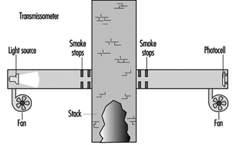
By using different light sources and detectors such as ultraviolet light (UV), gases transparent to visible light can be detected. These devices can be tuned to specific gases, and thus can measure gas concentration in the waste stream.

An in situ monitoring system has an advantage over an extractive system in that it can measure the concentration across the entire stack or duct, whereas the extractive method measures concentrations only at the point from which the sample was extracted. This can result in significant error if the sample gas stream is not well mixed. However, the extractive method offers more methods of analysis, and thus perhaps can be used in more applications.

Since the in situ system provides a continuous readout, it can be used to document emissions, or to fine tune the operating system.

Back

Air quality monitoring means the systematic measurement of ambient air pollutants in order to be able to assess the exposure of vulnerable receptors (e.g., people, animals, plants and art works) on the basis of standards and guidelines derived from observed effects, and/or to establish the source of the air pollution (causal analysis).

Ambient air pollutant concentrations are influenced by the spatial or time variance of emissions of hazardous substances and the dynamics of their dispersion in the air. As a consequence, marked daily and annual variations of concentrations occur. It is practically impossible to determine in a unified way all these different variations of air quality (in statistical language, the population of air quality states). Thus, ambient air pollutant concentrations measurements always have the character of random spatial or time samples.

Measurement Planning

The first step in measurement planning is to formulate the purpose of the measurement as precisely as possible. Important questions and fields of operation for air quality monitoring include:

Area measurement:

• representative determination of exposure in one area (general air monitoring)
• representative measurement of pre-existing pollution in the area of a planned facility (permit, TA Luft (Technical instruction, air))
• smog warning (winter smog, high ozone concentrations)
• measurements in hot spots of air pollution to estimate maximum exposure of receptors (EU-NO₂ guideline, measurements in street canyons, in accordance with the German Federal Immission Control Act)
• checking the results of pollution abatement measures and trends over time
• screening measurements
• scientific investigations - for example, the transport of air pollution, chemical conversions, calibrating dispersion calculations.

Facility measurement:

• measurements in response to complaints
• ascertaining sources of emissions, causal analysis
• measurements in cases of fires and accidental releases
• checking success of reduction measures
• monitoring factory fugitive emissions.

The goal of measurement planning is to use adequate measurement and assessment procedures to answer specific questions with sufficient certainty and at minimum possible expense.

An example of the parameters that should be used for measurement planning is presented in table 1, in relation to an assessment of air pollution in the area of a planned industrial facility. Recognizing that formal requirements vary by jurisdiction, it should be noted that specific reference here is made to German licensing procedures for industrial facilities.

Table 1. Parameters for measurement planning in measuring ambient air pollution concentrations (with example of application)

The example in table 1 shows the case of a measurement network that is supposed to monitor the air quality in a specific area as representatively as possible, to compare with designated air quality limits. The idea behind this approach is that a random choice of measurement sites is made in order to cover equally locations in an area with varying air quality (e.g., living areas, streets, industrial zones, parks, city centres, suburbs). This approach may be very costly in large areas due to the number of measurement sites necessary.

Another conception for a measurement network therefore starts with measurement sites that are representatively selected. If measurements of differing air quality are conducted in the most important locations, and the length of time that the protected objects remain in these “microenvironments” is known, then the exposure can be determined. This approach can be extended to other microenvironments (e.g., interior rooms, cars) in order to estimate the total exposure. Diffusion modelling or screening measurements can help in choosing the right measurement sites.

A third approach is to measure at the points of presumed highest exposure (e.g., for NO₂ and benzene in street canyons). If assessment standards are met at this site, there is sufficient probability that this will also be the case for all other sites. This approach, by focusing on critical points, requires relatively few measurement sites, but these must be chosen with particular care. This particular method risks overestimating real exposure.

The parameters of measurement time period, assessment of the measurement data and measurement frequency are essentially given in the definition of the assessment standards (limits) and the desired level of certainty of the results. Threshold limits and the peripheral conditions to be considered in measurement planning are related. By using continuous measurement procedures, a resolution that is temporally almost seamless can be achieved. But this is necessary only in monitoring peak values and/or for smog warnings; for monitoring annual mean values, for example, discontinuous measurements are adequate.

The following section is dedicated to describing the capabilities of measurement procedures and quality control as a further parameter important to measurement planning.

Quality Assurance

Measurements of ambient air pollutant concentrations can be costly to conduct, and results can affect significant decisions with serious economic or ecological implications. Therefore, quality assurance measures are an integral part of the measurement process. Two areas should be distinguished here.

Procedure-oriented measures

Every complete measurement procedure consists of several steps: sampling, sample preparation and clean-up; separation, detection (final analytical step); and data collection and assessment. In some cases, especially with continuous measurement of inorganic gases, some steps of the procedure can be left out (e.g., separation). Comprehensive adherence to procedures should be strived for in conducting measurements. Procedures that are standardized and thus comprehensively documented should be followed, in the form of DIN/ISO standards, CEN standards or VDI guidelines.

User-oriented measures

Using standardized and proven equipment and procedures for ambient air pollutant concentration measurement cannot alone ensure acceptable quality if the user does not employ adequate methods of quality control. The standards series DIN/EN/ISO 9000 (Quality Management and Quality Assurance Standards), EN 45000 (which defines the requirements for testing laboratories) and ISO Guide 25 (General Requirements for the Competence of Calibration and Testing Laboratories) are important for user-oriented measures to ensure quality.

Important aspects of user quality control measures include:

• acceptance and practice of the content of the measures in the sense of good laboratory practice (GLP)
• correct maintenance of measurement equipment, qualified measures to eliminate disruptions and ensure repairs
• carrying out calibrations and regular checking to ensure proper functioning
• carrying out interlaboratory testing.

Measurement Procedures

Measurement procedures for inorganic gases

A wealth of measurement procedures exists for the broad range of inorganic gases. We will differentiate between manual and automatic methods.

Manual procedures

In the case of manual measurement procedures for inorganic gases, the substance to be measured is normally adsorbed during the sampling in a solution or solid material. In most cases a photometric determination is made after an appropriate colour reaction. Several manual measurement procedures have special significance as reference procedures. Because of the relatively high personnel cost, these manual procedures are conducted only rarely for field measurements today, when alternative automatic procedures are available. The most important procedures are briefly sketched in table 2.

Table 2. Manual measurement procedures for inorganic gases

DL = detection limit; s = standard deviation; rel. s = relative s.

A special sampling variant, used primarily in connection with manual measurement procedures, is the diffusion separation tube (denuder). The denuder technique is aimed at separating the gas and particle phases by using their different diffusion rates. Thus, it is often used on difficult separation problems (e.g., ammonia and ammonium compounds; nitrogen oxides, nitric acid and nitrates; sulphur oxides, sulphuric acid and sulphates or hydrogen halides/halides). In the classic denuder technique, the test air is sucked through a glass tube with a special coating, depending on the material(s) to be collected. The denuder technique has been further developed in many variations and also partially automated. It has greatly expanded the possibilities of differentiated sampling, but, depending on the variant, it can be very laborious, and proper utilization requires a great deal of experience.

Automated procedures

There are numerous different continuous measuring monitors on the market for sulphur dioxide, nitrogen oxides, carbon monoxide and ozone. For the most part they are used particularly in measurement networks. The most important features of the individual methods are collected in table 3.

Table 3. Automated measurement procedures for inorganic gases

It should be emphasized here that all automatic measurement procedures based on chemical-physical principles must be calibrated using (manual) reference procedures. Since automatic equipment in measurement networks often runs for extended periods of time (e.g., several weeks) without direct human supervision, it is indispensable that their correct functioning is regularly and automatically checked. This generally is done using zero and test gases that can be produced by several methods (preparation of ambient air; pressurized gas cylinders; permeation; diffusion; static and dynamic dilution).

Measurement procedures for dust-forming air pollutants and its composition

Among particulate air pollutants, dustfall and suspended particulate matter (SPM) are differentiated. Dustfall consists of larger particles, which sink to the ground because of their size and thickness. SPM includes the particle fraction that is dispersed in the atmosphere in a quasi-stable and quasi-homogenous manner and therefore remains suspended for a certain time.

Measurement of suspended particulate matter and metallic compounds in SPM

As is the case with measurements of gaseous air pollutants, continuous and discontinuous measurement procedures for SPM can be differentiated. As a rule, SPM is first separated on glass fibre or membrane filters. It follows a gravimetric or radiometric determination. Depending on the sampling, a distinction can be made between a procedure to measure the total SPM without fractionation according to the size of the particles and a fractionation procedure to measure the fine dust.

The advantages and disadvantages of fractionated suspended dust measurements are disputed internationally. In Germany, for example, all threshold limits and assessment standards are based on total suspended particulates. This means that, for the most part, only total SPM measurements are performed. In the United States, on the contrary, the so-called PM-10 procedure (particulate matter £ 10μm) is very common. In this procedure, only particles with an aerodynamic diameter up to 10 μm are included (50 per cent inclusion portion), which are inhalable and can enter the lungs. The plan is to introduce the PM-10 procedure into the European Union as a reference procedure. The cost for fractionated SPM measurements is considerably higher than for measuring total suspended dust, because the measuring devices must be fitted with special, expensively constructed sampling heads that require costly maintenance. Table 4 contains details on the most important SPM measurement procedures.

Table 4. Measurement procedures for suspended particulate matter (SPM)

Recently, automatic filter changers have also been developed that hold a larger number of filters and supply them to the sampler, one after another, at timed intervals. The exposed filters are stored in a magazine. The detection limits for filter procedures lie between 5 and 10 μg/m³ of dust, as a rule.

Finally, the black smoke procedure for SPM measurements has to be mentioned. Coming from Britain, it has been incorporated into EU guidelines for SO₂ and suspended dust. In this procedure, the blackening of the coated filter is measured with a reflex photometer after the sampling. The black smoke values that are thus photometrically obtained are converted into gravimetric units (μg/m³) with the help of a calibration curve. Since this calibration function depends to a high degree on the composition of the dust, especially its soot content, the conversion into gravimetric units is problematic.

Today, metal compounds are often routinely determined in suspended dust immission samples. In general, the collection of the suspended dust on filters is followed by a chemical dissolution of the separated dusts, since the most common final analytical steps presuppose converting the metallic and metalloid compounds in an aqueous solution. In practice, the most important methods by far are atom absorption spectroscopy (AAS) and spectroscopy with plasma excitation (ICP-OES). Other procedures for determining metallic compounds in suspended dust are x-ray fluorescence analysis, polarography and neutron activation analysis. Although metallic compounds have been measured for more than a decade now as a component of SPM in outside air at certain measurement sites, important unanswered questions remain. Thus the conventional sampling by separating the suspended dust on filters assumes that the separation of the heavy metal compounds on the filter is complete. However, earlier indications have been found in the literature questioning this. The results are very heterogeneous.

A further problem lies in the fact that different compound forms, or single compounds of the respective elements, cannot be distinguished in the analysis of metallic compounds in suspended dust using the conventional measurement procedures. While in many cases adequate total determinations can be made, a more thorough differentiation would be desirable with certain especially carcinogenic metals (As, Cd, Cr, Ni, Co, Be). There are often big differences in the carcinogenic effects of elements and their individual compounds (e.g., chromium compounds in oxidation levels III and VI - only those in level VI are carcinogenic). In such cases a specific measurement of the individual compounds (species analysis) would be desirable. Despite the significance of this problem, only first attempts at species analysis are being made in measurement technique.

Measurement of dustfall and metallic compounds in dustfall

Two fundamentally different methods are used to collect dustfall:

• sampling in collecting vessels

• sampling on adhesive surfaces.

A popular procedure for measuring dustfall (deposited dust) is the so-called Bergerhoff procedure. In this procedure the entire atmospheric precipitation (dry and wet depositions) is collected over 30± 2 days in vessels about 1.5 to 2.0 metres above the ground (bulk deposition). Then the collecting vessels are taken to the lab and prepared (filtered, water evaporated, dried, weighed). The result is calculated on the basis of the surface area of the collecting vessel and exposure time in grams per square meter and day (g/m²d). The relative detection limit is 0.035 g/m²d.

Additional procedures for collecting dustfall include the Liesegang-Löbner device and methods which collect the deposited dust on adhesive foils.

All measurement results for dustfall are relative values that depend on the apparatus used, as the dust separation is influenced by the flow conditions at the device and other parameters. The differences in the measurement values obtained with the different procedures can reach 50 per cent.

Also important is the composition of the deposited dust, such as the content of lead, cadmium and other metallic compounds. The analytical procedures used for this are basically the same as those used for suspended dust.

Measuring special materials in dust form

Special materials in dust form include asbestos and soot. Collecting fibres as air pollutants is important since asbestos has been classified as a confirmed carcinogenic material. Fibres with a diameter of D ≤ 3μm and a length of L ≥ 5μm, where L:D ≥ 3, are considered carcinogenic. Measurement procedures for fibrous materials consist of counting, under the microscope, fibres that have been separated on filters. Only electron microscopic procedures can be considered for outside air measurements. The fibres are separated on gold-coated porous filters. Prior to assessment in an electron scan microscope, the sample is freed of organic substances through plasma incineration right on the filter. The fibres are counted on part of the filter surface, randomly chosen and classified by geometry and type of fibre. With the help of energy dispersive x-ray analysis (EDXA), asbestos fibres, calcium sulphate fibres and other inorganic fibres can be differentiated on the basis of elemental composition. The entire procedure is extremely expensive and requires the greatest care to achieve reliable results.

Soot in the form of particles emitted by diesel motors has become relevant since diesel soot was also classified as carcinogenic. Because of its changing and complex composition and because of the fact that various constituents are also emitted from other sources, there is no measurement procedure specific to diesel soot. Nevertheless, in order to say something concrete about the concentrations in ambient air, soot is conventionally defined as elemental carbon, as a part of total carbon. It is measured after sampling and an extraction step and/or thermal desorption. Determination of the carbon content ensues through burning in an oxygen stream and coulometric titration or non-dispersive IR detection of the carbon dioxide formed in the process.

The so-called aethalometer and the photoelectric aerosol sensor are also used for measuring soot, in principle.

Measuring Wet Depositions

Together with dry deposition, wet deposition in rain, snow, fog and dew constitute the most important means by which harmful materials enter the ground, water or plant surfaces from the air.

In order to clearly distinguish the wet deposition in rain and snow (fog and dew present special problems) from the measurement of total deposition (bulk deposition, see section “Measurement of dustfall and metallic compounds” above) and dry deposition, rain catchers, whose collection opening is covered when there is no rain (wet-only sampler), are used for sampling. With rain sensors, which mostly work on the principle of conductivity changes, the cover is opened when it starts to rain and closed again when the rain stops.

The samples are transferred through a funnel (open area approx. 500 cm² and more) into a darkened and if possible insulated collection container (of glass or polyethylene for inorganic components only).

In general, analysing the collected water for inorganic components can be done without sample preparation. The water should be centrifuged or filtered if it is visibly cloudy. The conductivity, pH value and important anions (NO₃ ^– , SO₄ ^2– , Cl^–) and cations (Ca²⁺, K⁺, Mg²⁺, Na⁺, NH₄ ⁺ and so on) are routinely measured. Unstable trace compounds and intermediate states like H₂O₂ or HSO₃ ^– are also measured for research purposes.

For analysis, procedures are used that are generally available for aqueous solutions such as conductometry for conductivity, electrodes for pH values, atom adsorption spectroscopy for cations (see section “Measuring special materials in dust form”, above) and, increasingly, ion exchange chromatography with conductivity detection for anions.

Organic compounds are extracted from rain water with, for example, dichloromethane, or blown out with argon and adsorbed with Tenax tubes (only highly volatile materials). The materials are then subjected to a gas chromatographic analysis (see “Measurement procedures for organic air pollutants”, below).

Dry deposition correlates directly with ambient air concentrations. The concentration differences of airborne harmful materials in rain, however, are relatively small, so that for measuring wet deposition, wide-mesh measuring networks are adequate. Examples include the European EMEP measurement network, in which the entry of sulphate and nitrate ions, certain cations and precipitation pH values are collected in approximately 90 stations. There are also extensive measurement networks in North America.

Optical Long-Distance Measurement Procedures

Whereas the procedures described up to now catch air pollution at one point, optical long-distance measuring procedures measure in an integrated manner over light paths of several kilometres or they determine the spatial distribution. They use the absorption characteristics of gases in the atmosphere in the UV, visible or IR spectral range and are based on the Lambert-Beer law, according to which the product of light path and concentration are proportional to the measured extinction. If the sender and receiver of the measuring installation change the wavelength, several components can be measured in parallel or sequentially with one device.

In practice, the measurement systems identified in table 5 play the biggest role.

Table 5. Long-distance measurement procedures

LIDAR = Light detection and ranging; DIAL = differential absorption LIDAR.

Measurement Procedures for Organic Air Pollutants

The measurement of air pollution containing organic components is complicated primarily by the range of materials in this class of compounds. Several hundred individual components with very different toxicological, chemical and physical characteristics are covered under the general title “organic air pollutants” in the emissions registers and air quality plans of congested areas.

Especially due to the great differences in potential impact, collecting relevant individual components has more and more taken the place of previously used summation procedures (e.g., Flame Ionization Detector, total carbon procedure), the results of which cannot be assessed toxicologically. The FID method, however, has retained a certain significance in connection with a short separation column to separate out methane, which is photochemically not very reactive, and for collecting the precursor volatile organic compounds (VOC) for the formation of photo-oxidants.

The frequent necessity of separating the complex mixtures of the organic compounds into relevant individual components makes measuring it virtually an exercise in applied chromatography. Chromatographic procedures are the methods of choice when the organic compounds are sufficiently stable, thermally and chemically. For organic materials with reactive functional groups, separate procedures that use the functional groups’ physical characteristics or chemical reactions for detection continue to hold their ground.

Examples include using amines to convert aldehydes to hydrazones, with subsequent photometric measurement; derivatization with 2,4-dinitrophenylhydrazine and separation of the 2,4-hydrazone that is formed; or forming azo-dyes with p-nitroaniline for detecting phenols and cresols.

Among chromatographic procedures, gas chromatography (GC) and high-pressure liquid chromatography (HPLC) are most frequently employed for separating the often complex mixtures. For gas chromatography, separation columns with very narrow diameters (approx. 0.2 to 0.3 mm, and approx. 30 to 100 m long), so-called high-resolution capillary columns (HRGC), are almost exclusively utilized today. A series of detectors are available for finding the individual components after the separation column, such as the above-mentioned FID, the ECD (electron capture detector, specifically for electrophilic substitutes such as halogen), the PID (photo-ionization detector, which is especially sensitive to aromatic hydrocarbons and other p-electron systems), and the NPD (thermo-ionic detector specifically for nitrogen and phosphorus compounds). The HPLC uses special through-flow detectors which, for example, are designed as the through-flow cuvette of a UV spectrometer.

Especially effective, but also especially expensive, is the use of a mass spectrometer as a detector. Really certain identification, especially with unknown mixtures of compounds, is often possible only through the mass spectrum of the organic compound. The qualitative information of the so-called retention time (time the material remains in the column) that is contained in the chromatogram with conventional detectors is supplemented with the specific detection of the individual components by mass fragmentograms with high detection sensitivity.

Sampling must be considered before the actual analysis. The choice of sampling method is determined primarily by volatility, but also by expected concentration range, polarity and chemical stability. Furthermore, with non-volatile compounds, a choice must be made between concentration and deposition measurements.

Table 6 provides an overview of common procedures in air monitoring for active enrichment and chromatographic analysis of organic compounds, with examples of applications.

Table 6. Overview of common chromatographic air quality measurement procedures of organic compounds (with examples of applications)

GC = gas chromatography; GCMS = GC/mass spectroscopy; FID = flame ionization detector; HRGC/ECD = high resolution GC/ECD; ECD = electron capture detector; HPLC = high performance liquid chromatography. PID = photo-ionization detector.

Deposition measurements of organic compounds with low volatility (e.g., dibenzodioxins and dibenzofurans (PCDD/PCDF), polycyclic aromatic hydrocarbons (PAH)) are gaining in importance from the perspective of environmental impact. Since food is the main source of human intake, airborne material transferred onto food plants is of great significance. There is, however, evidence that material transfer by way of particulate deposition is less important than dry deposition of quasi-gaseous compounds.

For measuring total deposition, standardized devices for dust precipitation are used (e.g., Bergerhoff procedure), which have been slightly modified by darkening as a protection against the entry of strong light. Important technical measurement problems, such as the resuspension of already separated particles, evaporation or possible photolytic decomposition, are now being systematically researched in order to improve the less-than-optimal sampling procedures for organic compounds.

Olfactometric Investigations

Olfactometric immission investigations are used in monitoring to quantify odour complaints and to determine baseline pollution in licensing procedures. They serve primarily to assess whether existing or anticipated odours should be classified as significant.

In principle, three methodological approaches can be differentiated:

• measurement of the emission concentration (number of odour units) with an olfactometer and subsequent dispersion modelling

• measurement of individual components (e.g., NH₃) or mixtures of compounds (e.g., gas chromatography of gases from landfills), if these adequately characterize the odour

• odour determinations by means of inspections.

The first possibility combines emission measurement with modelling and, strictly speaking, cannot be classified under the term air quality monitoring. In the third method, the human nose is used as the detector with significantly reduced precision as compared to physical-chemical methods.

Details of inspections, measurement plans and assessing the results are contained, for example, in the environmental protection regulations of some German states.

Screening Measurement Procedures

Simplified measurement procedures are sometimes used for preparatory studies (screening). Examples include passive samplers, test tubes and biological procedures. With passive (diffusive) samplers, the material to be tested is collected with freely flowing processes such as diffusion, permeation or adsorption in simple forms of collectors (tubes, plaques) and enriched in impregnated filters, meshes or other adsorption media. So-called active sampling (sucking the sample air through a pump) thus does not occur. The enriched quantity of material, analytically determined according to definite exposure time, is converted into concentration units on the basis of physical laws (e.g., of diffusion) with the help of collection time and the collector’s geometric parameters. The methodology stems from the field of occupational health (personal sampling) and indoor air measurement, but it is increasingly being used for ambient air pollutant concentration measurements. An overview can be found in Brown 1993.

Detector tubes are often used for sampling and quick preparatory analysis of gases. A certain test air volume is sucked through a glass tube that is filled with an adsorptive reagent that corresponds with the test objective. The contents of the tube change colour depending on the concentration of the material to be determined that is present in the test air. Small testing tubes are often used in the field of workplace monitoring or as a quick procedure in cases of accidents, such as fires. They are not used for routine ambient air pollutant concentration measurements due to the generally too high detection limits and too limited selectivity. Detector testing tubes are available for numerous materials in various concentration ranges.

Among the biological procedures, two methods have become accepted in routine monitoring. With the standardized lichen exposure procedure, the mortality rate of the lichen is determined over the exposure time of 300 days. In another procedure, French pasture grass is exposed for 14±1 days. Then the amount of growth is determined. Both procedures serve as summary determinations of air pollutant concentration effects.

Air Quality Monitoring Networks

Around the world, the most varied types of air quality networks are utilized. A distinction should be drawn between measurement networks, consisting of automatic, computer-controlled measuring stations (measurement containers), and virtual measurement networks, which only define the measurement locations for various types of air pollutant concentration measurements in the form of a preset grid. Tasks and conceptions of measurement networks were discussed above.

Continuous monitoring networks

Continuously operating measurement networks are based on automatic measuring stations, and serve primarily for air quality monitoring of urban areas. Measured are air pollutants such as sulphur dioxide (SO₂), dust, nitrogen monoxide (NO), nitrogen dioxide (NO₂), carbon monoxide (CO), ozone (O₃), and to an extent also the sum of the hydrocarbons (free methane, C_nH_m) or individual organic components (e.g., benzene, toluene, xylenes). In addition, depending on need, meteorological parameters such as wind direction, wind speed, air temperature, relative humidity, precipitation, global radiation or radiation balance are included.

The measuring equipment operated in measurement stations generally consists of an analyser, a calibration unit, and control and steering electronics, which monitors the whole measuring equipment and contains a standardized interface for data collection. In addition to the measurement values, the measuring equipment supplies so-called status signals on errors and the operating status. The calibration of the devices is automatically checked by computer at regular intervals.

As a rule, the measurement stations are connected with fixed data lines, dial connections or other data transfer systems to a computer (process computer, workstation or PC, depending on the scope of the system) in which the measurement results are entered, processed and displayed. The measurement network computers and, if necessary, specially trained personnel monitor continuously whether various threshold limits are exceeded. In this manner critical air quality situations can be recognized at any time. This is very important, especially for monitoring critical smog situations in winter and summer (photo-oxidants) and for current public information.

Measurement networks for random sample measurements

Beyond the telemetric measurement network, other measuring systems for monitoring air quality are used to varying extents. Examples include (occasionally partially automated) measurement networks to determine:

• dust deposition and its components
• suspended dust (SPM) and its components
• hydrocarbons and chlorinated hydrocarbons
• low volatile organic materials (dioxins, furans, polychlorinated biphenyls).

A series of substances measured in this manner have been classified as carcinogens, such as cadmium compounds, PAHs or benzene. Monitoring them is therefore particularly important.

To provide an example of a comprehensive programme, table 7 summarizes the air quality monitoring that is systematically conducted in North Rhine-Westphalia, which with 18 million inhabitants is the most populous state in Germany.

Table 7. Systematic air quality monitoring in North-Rhine-Westphalia (Germany)

Back

The aim of air pollution modelling is the estimation of outdoor pollutant concentrations caused, for instance, by industrial production processes, accidental releases or traffic. Air pollution modelling is used to ascertain the total concentration of a pollutant, as well as to find the cause of extraordinary high levels. For projects in the planning stage, the additional contribution to the existing burden can be estimated in advance, and emission conditions may be optimized.

Figure 1. Global Environmental Monitoring System/Air pollution management

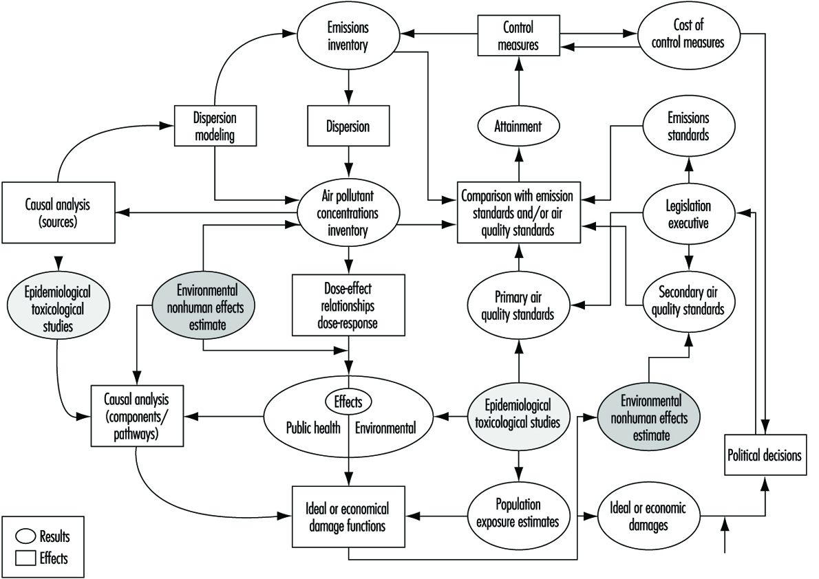
Depending on the air quality standards defined for the pollutant in question, annual mean values or short-time peak concentrations are of interest. Usually concentrations have to be determined where people are active - that is, near the surface at a height of about two metres above the ground.

Parameters Influencing Pollutant Dispersion

Two types of parameters influence pollutant dispersion: source parameters and meteorological parameters. For source parameters, concentrations are proportional to the amount of pollutant which is emitted. If dust is concerned, the particle diameter has to be known to determine sedimentation and deposition of the material (VDI 1992). As surface concentrations are lower with greater stack height, this parameter also has to be known. In addition, concentrations depend on the total amount of the exhaust gas, as well as on its temperature and velocity. If the temperature of the exhaust gas exceeds the temperature of the surrounding air, the gas will be subject to thermal buoyancy. Its exhaust velocity, which can be calculated from the inner stack diameter and the exhaust gas volume, will cause a dynamic momentum buoyancy. Empirical formulae may be used to describe these features (VDI 1985; Venkatram and Wyngaard 1988). It has to be stressed that it is not the mass of the pollutant in question but that of the total gas that is responsible for the thermal and dynamic momentum buoyancy.

Meteorological parameters which influence pollutant dispersion are wind speed and direction, as well as vertical thermal stratification. The pollutant concentration is proportional to the reciprocal of wind speed. This is mainly due to the accelerated transport. Moreover, turbulent mixing increases with growing wind speed. As so-called inversions (i.e., situations where temperature is increasing with height) hinder turbulent mixing, maximum surface concentrations are observed during highly stable stratification. On the contrary, convective situations intensify vertical mixing and therefore show the lowest concentration values.

Air quality standards - for example, annual mean values or 98 percentiles - are usually based on statistics. Hence, time series data for the relevant meteorological parameters are needed. Ideally, statistics should be based on ten years of observation. If only shorter time series are available, it should be ascertained that they are representative for a longer period. This can be done, for example, by analysis of longer time series from other observations sites.

The meteorological time series used also has to be representative of the site considered - that is, it must reflect the local characteristics. This is specially important concerning air quality standards based on peak fractions of the distribution, like 98 percentiles. If no such time series is at hand, a meteorological flow model may be used to calculate one from other data, as will be described below.

The Global Atmospheric Watch (GAW) programme (Miller and Soudine 1994) provides data and other information on the chemical composition and related physical characteristics of the atmosphere, and their trends, with the objective of understanding the relationship between changing atmospheric composition and changes of global and regional climate, the long-range atmospheric transport and deposition of potentially harmful substances over terrestrial, fresh-water and marine ecosystems, and the natural cycling of chemical elements in the global atmosphere/ocean/biosphere system, and anthropogenic impacts thereon. The GAW programme consists of four activity areas: the Global Ozone Observing System (GO3OS), global monitoring of background atmospheric composition, including the Background Air Pollution Monitoring Network (BAPMoN); dispersion, transport, chemical transformation and deposition of atmospheric pollutants over land and sea on different time and space scales; exchange of pollutants between the atmosphere and other environmental compartments; and integrated monitoring. One of the most important aspects of the GAW is the establishment of Quality Assurance Science Activity Centres to oversee the quality of the data produced under GAW.

Concepts of Air Pollution Modelling

As mentioned above, dispersion of pollutants is dependent on emission conditions, transport and turbulent mixing. Using the full equation which describes these features is called Eulerian dispersion modelling (Pielke 1984). By this approach, gains and losses of the pollutant in question have to be determined at every point on an imaginary spatial grid and in distinct time steps. As this method is very complex and computer time consuming, it usually cannot be handled routinely. However, for many applications, it may be simplified using the following assumptions:

• no change of emission conditions with time

• no change of meteorological conditions during transport

• wind speeds above 1 m/s.

In this case, the equation mentioned above can be solved analytically. The resulting formula describes a plume with Gaussian concentration distribution, the so called Gaussian plume model (VDI 1992). The distribution parameters depend on meteorological conditions and downwind distance as well as on stack height. They have to be determined empirically (Venkatram and Wyngaard 1988). Situations where emissions and/or meteorological parameters vary by a considerable amount in time and/or space may be described by the Gaussian puff model (VDI 1994). Under this approach, distinct puffs are emitted in fixed time steps, each following its own path according to the current meteorological conditions. On its way, each puff grows according to turbulent mixing. Parameters describing this growth, again, have to be determined from empirical data (Venkatram and Wyngaard 1988). It has to be stressed, however, that to achieve this objective, input parameters must be available with the necessary resolution in time and/or space.

Concerning accidental releases or single case studies, a Lagrangian or particle model (VDI Guideline 3945, Part 3) is recommended. The concept thereby is to calculate the paths of many particles, each of which represents a fixed amount of the pollutant in question. The individual paths are composed of transport by the mean wind and of stochastic disturbances. Due to the stochastic part, the paths do not fully agree, but depict the mixture by turbulence. In principle, Lagrangian models are capable of considering complex meteorological conditions - in particular, wind and turbulence; fields calculated by flow models described below can be used for Lagrangian dispersion modelling.

Dispersion Modelling in Complex Terrain

If pollutant concentrations have to be determined in structured terrain, it may be necessary to include topographic effects on pollutant dispersion in modelling. Such effects are, for example, transport following the topographic structure, or thermal wind systems like sea breezes or mountain winds, which change wind direction in the course of the day.

If such effects take place on a scale much larger than the model area, the influence may be considered by using meteorological data which reflect the local characteristics. If no such data are available, the three-dimensional structure impressed on the flow by topography can be obtained by using a corresponding flow model. Based on these data, dispersion modelling itself may be carried out assuming horizontal homogeneity as described above in the case of the Gaussian plume model. However, in situations where wind conditions change significantly inside the model area, dispersion modelling itself has to consider the three-dimensional flow affected by the topographic structure. As mentioned above, this may be done by using a Gaussian puff or a Lagrangian model. Another way is to perform the more complex Eulerian modelling.

To determine wind direction in accord with the topographically structured terrain, mass consistent or diagnostic flow modelling may be used (Pielke 1984). Using this approach, the flow is fitted to topography by varying the initial values as little as possible and by keeping its mass consistent. As this is an approach which leads to quick results, it may also be used to calculate wind statistics for a certain site if no observations are available. To do this, geostrophic wind statistics (i.e., upper air data from rawinsondes) are used.

If, however, thermal wind systems have to be considered in more detail, so called prognostic models have to be used. Depending on the scale and the steepness of the model area, a hydrostatic, or the even more complex non-hydrostatic, approach is suitable (VDI 1981). Models of this type need much computer power, as well as much experience in application. Determination of concentrations based on annual means, in general, are not possible with these models. Instead, worst case studies can be performed by considering only one wind direction and those wind speed and stratification parameters which result in the highest surface concentration values. If those worst case values do not exceed air quality standards, more detailed studies are not necessary.

Figure 2. Topographic structure of a model region

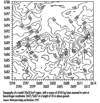
Figure 2, figure 3 and figure 4 demonstrate how the transport and dispension of pollutants can be presented in relation to the influence of terrain and wind climatologies derived from consideration of surface and geostrophic wind frequencies.

Figure 3. Surface frequency distributions as determined from geostrophic  frequency distribution

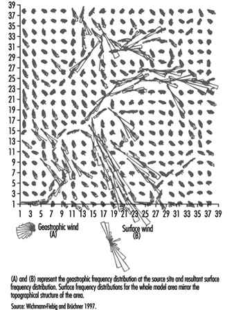
Figure 4.  Annual mean pollutant concentrations for a hypothetical region calculated  from the geostrophic frequency distribution for heterogeneous wind fields

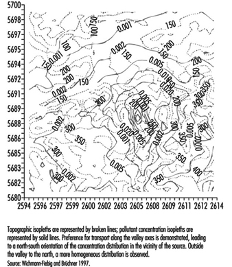
Dispersion Modelling in Case of Low Sources

Considering air pollution caused by low sources (i.e., stack heights on the order of building height or emissions of road traffic) the influence of the surrounding buildings has to be considered. Road traffic emissions will be trapped to a certain amount in street canyons. Empirical formulations have been found to describe this (Yamartino and Wiegand 1986).

Pollutants emitted from a low stack situated on a building will be captured in the circulation on the lee side of the building. The extent of this lee circulation depends on the height and width of the building, as well as on wind speed. Therefore, simplified approaches to describe pollutant dispersion in such a case, based solely on the height of a building, are not generally valid. The vertical and horizontal extent of the lee circulation has been obtained from wind tunnel studies (Hosker 1985) and can be implemented in mass consistent diagnostic models. As soon as the flow field has been determined, it can be used to calculate the transport and turbulent mixing of the pollutant emitted. This can be done by Lagrangian or Eulerian dispersion modelling.

More detailed studies - concerning accidental releases, for instance - can be performed only by using non-hydrostatic flow and dispersion models instead of a diagnostic approach. As this, in general, demands high computer power, a worst case approach as described above is recommended in advance of a complete statistical modelling.

Back

Air pollution management aims at the elimination, or reduction to acceptable levels, of airborne gaseous pollutants, suspended particulate matter and physical and, to a certain extent, biological agents whose presence in the atmosphere can cause adverse effects on human health (e.g., irritation, increase of incidence or prevalence of respiratory diseases, morbidity, cancer, excess mortality) or welfare (e.g., sensory effects, reduction of visibility), deleterious effects on animal or plant life, damage to materials of economic value to society and damage to the environment (e.g., climatic modifications). The serious hazards associated with radioactive pollutants, as well as the special procedures required for their control and disposal, also deserve careful attention.

The importance of efficient management of outdoor and indoor air pollution cannot be overemphasized. Unless there is adequate control, the multiplication of pollution sources in the modern world may lead to irreparable damage to the environment and mankind.

The objective of this article is to give a general overview of the possible approaches to the management of ambient air pollution from motor vehicle and industrial sources. However, it is to be emphasized from the very beginning that indoor air pollution (in particular, in developing countries) might play an even larger role than outdoor air pollution due to the observation that indoor air pollutant concentrations are often substantially higher than outdoor concentrations.

Beyond considerations of emissions from fixed or mobile sources, air pollution management involves consideration of additional factors (such as topography and meteorology, and community and government participation, among many others) all of which must be integrated into a comprehensive programme. For example, meteorological conditions can greatly affect the ground-level concentrations resulting from the same pollutant emission. Air pollution sources may be scattered over a community or a region and their effects may be felt by, or their control may involve, more than one administration. Furthermore, air pollution does not respect any boundaries, and emissions from one region may induce effects in another region by long-distance transport.

Air pollution management, therefore, requires a multidisciplinary approach as well as a joint effort by private and governmental entities.

Sources of Air Pollution

The sources of man-made air pollution (or emission sources) are of basically two types:

• stationary, which can be subdivided into area sources such as agricultural production, mining and quarrying, industrial, point and area sources such as manufacturing of chemicals, nonmetallic mineral products, basic metal industries, power generation and community sources (e.g., heating of homes and buildings, municipal waste and sewage sludge incinerators, fireplaces, cooking facilities, laundry services and cleaning plants)
• mobile, comprising any form of combustion-engine vehicles (e.g., light-duty gasoline powered cars, light- and heavy-duty diesel powered vehicles, motorcycles, aircraft, including line sources with emissions of gases and particulate matter from vehicle traffic).

In addition, there are also natural sources of pollution (e.g., eroded areas, volcanoes, certain plants which release great amounts of pollen, sources of bacteria, spores and viruses). Natural sources are not discussed in this article.

Types of Air Pollutants

Air pollutants are usually classified into suspended particulate matter (dusts, fumes, mists, smokes), gaseous pollutants (gases and vapours) and odours. Some examples of usual pollutants are presented below:

Suspended particulate matter (SPM, PM-10) includes diesel exhaust, coal fly-ash, mineral dusts (e.g., coal, asbestos, limestone, cement), metal dusts and fumes (e.g., zinc, copper, iron, lead) and acid mists (e.g., sulphuric acid), fluorides, paint pigments, pesticide mists, carbon black and oil smoke. Suspended particulate pollutants, besides their effects of provoking respiratory diseases, cancers, corrosion, destruction of plant life and so on, can also constitute a nuisance (e.g., accumulation of dirt), interfere with sunlight (e.g., formation of smog and haze due to light scattering) and act as catalytic surfaces for reaction of adsorbed chemicals.

Gaseous pollutants include sulphur compounds (e.g., sulphur dioxide (SO₂) and sulphur trioxide (SO₃)), carbon monoxide, nitrogen compounds (e.g., nitric oxide (NO), nitrogen dioxide (NO₂), ammonia), organic compounds (e.g., hydrocarbons (HC), volatile organic compounds (VOC), polycyclic aromatic hydrocarbons (PAH), aldehydes), halogen compounds and halogen derivatives (e.g., HF and HCl), hydrogen sulphide, carbon disulphide and mercaptans (odours).

Secondary pollutants may be formed by thermal, chemical or photochemical reactions. For example, by thermal action sulphur dioxide can oxidize to sulphur trioxide which, dissolved in water, gives rise to the formation of sulphuric acid mist (catalysed by manganese and iron oxides). Photochemical reactions between nitrogen oxides and reactive hydrocarbons can produce ozone (O₃), formaldehyde and peroxyacetyl nitrate (PAN); reactions between HCl and formaldehyde can form bis-chloromethyl ether.

While some odours are known to be caused by specific chemical agents such as hydrogen sulphide (H₂S), carbon disulphide (CS₂) and mercaptans (R-SH or R1-S-R2) others are difficult to define chemically.

Examples of the main pollutants associated with some industrial air pollution sources are presented in table 1 (Economopoulos 1993).

Table 1. Common atmospheric pollutants and their sources

Source: Economopoulos 1993

Clean Air Implementation Plans

Air quality management aims at the preservation of environmental quality by prescribing the tolerated degree of pollution, leaving it to the local authorities and polluters to devise and implement actions to ensure that this degree of pollution will not be exceeded. An example of legislation within this approach is the adoption of ambient air quality standards based, very often, on air quality guidelines (WHO 1987) for different pollutants; these are accepted maximum levels of pollutants (or indicators) in the target area (e.g., at ground level at a specified point in a community) and can be either primary or secondary standards. Primary standards (WHO 1980) are the maximum levels consistent with an adequate safety margin and with the preservation of public health, and must be complied with within a specific time limit; secondary standards are those judged to be necessary for protection against known or anticipated adverse effects other than health hazards (mainly on vegetation) and must be complied “within a reasonable time”. Air quality standards are short-, medium- or long-term values valid for 24 hours per day, 7 days per week, and for monthly, seasonal or annual exposure of all living subjects (including sensitive subgroups such as children, the elderly and the sick) as well as non-living objects; this is in contrast to maximum permissible levels for occupational exposure, which are for a partial weekly exposure (e.g., 8 hours per day, 5 days per week) of adult and supposedly healthy workers.

Typical measures in air quality management are control measures at the source, for example, enforcement of the use of catalytic converters in vehicles or of emission standards in incinerators, land-use planning and shut-down of factories or reduction of traffic during unfavourable weather conditions. The best air quality management stresses that the air pollutant emissions should be kept to a minimum; this is basically defined through emission standards for single sources of air pollution and could be achieved for industrial sources, for example, through closed systems and high-efficiency collectors. An emission standard is a limit on the amount or concentration of a pollutant emitted from a source. This type of legislation requires a decision, for each industry, on the best means of controlling its emissions (i.e., fixing emission standards).

The basic aim of air pollution management is to derive a clean air implementation plan (or air pollution abatement plan) (Schwela and Köth-Jahr 1994) which consists of the following elements:

• description of area with respect to topography, meteorology and socioeconomy
• emissions inventory
• comparison with emission standards
• air pollutant concentrations inventory
• simulated air pollutant concentrations
• comparison with air quality standards
• inventory of effects on public health and the environment
• causal analysis
• control measures
• cost of control measures
• cost of public health and environmental effects
• cost-benefit analysis (costs of control vs. costs of efforts)
• transportation and land-use planning
• enforcement plan; resource commitment
• projections for the future on population, traffic, industries and fuel consumption
• strategies for follow-up.

Some of these issues will be described below.

Emissions Inventory; Comparison with Emission Standards

The emissions inventory is a most complete listing of sources in a given area and of their individual emissions, estimated as accurately as possible from all emitting point, line and area (diffuse) sources. When these emissions are compared with emission standards set for a particular source, first hints on possible control measures are given if emission standards are not complied with. The emissions inventory also serves to assess a priority list of important sources according to the amount of pollutants emitted, and indicates the relative influence of different sources—for example, traffic as compared to industrial or residential sources. The emissions inventory also allows an estimate of air pollutant concentrations for those pollutants for which ambient concentration measurements are difficult or too expensive to perform.

Air Pollutant Concentrations Inventory; Comparison with Air Quality Standards

The air pollutant concentrations inventory summarizes the results of the monitoring of ambient air pollutants in terms of annual means, percentiles and trends of these quantities. Compounds measured for such an inventory include the following:

• sulphur dioxide
• nitrogen oxides
• suspended particulate matter
• carbon monoxide
• ozone
• heavy metals (Pb, Cd, Ni, Cu, Fe, As, Be)
• polycyclic aromatic hydrocarbons: benzo(a)pyrene, benzo(e)pyrene, benzo(a)anthracene, dibenzo(a,h)anthracene, benzoghi)perylene, coronen
• volatile organic compounds: n-hexane, benzene, 3-methyl-hexane, n-heptane, toluene, octane, ethyl-benzene xylene (o-,m-,p-), n-nonane, isopropylbenzene, propylbenezene, n-2-/3-/4-ethyltoluene, 1,2,4-/1,3,5-trimethylbenzene, trichloromethane, 1,1,1 trichloroethane, tetrachloromethane, tri-/tetrachloroethene.

Comparison of air pollutant concentrations with air quality standards or guidelines, if they exist, indicates problem areas for which a causal analysis has to be performed in order to find out which sources are responsible for the non-compliance. Dispersion modelling has to be used in performing this causal analysis (see “Air pollution: Modelling of air pollutant dispersion”). Devices and procedures used in today’s ambient air pollution monitoring are described in “Air quality monitoring”.

Simulated Air Pollutant Concentrations; Comparison with Air Quality Standards

Starting from the emissions inventory, with its thousands of compounds which cannot all be monitored in the ambient air for economy reasons, use of dispersion modelling can help to estimate the concentrations of more “exotic” compounds. Using appropriate meteorology parameters in a suitable dispersion model, annual averages and percentiles can be estimated and compared to air quality standards or guidelines, if they exist.

Inventory of Effects on Public Health and the Environment; Causal Analysis

Another important source of information is the effects inventory (Ministerium für Umwelt 1993), which consists of results of epidemiological studies in the given area and of effects of air pollution observed in biological and material receptors such as, for example, plants, animals and construction metals and building stones. Observed effects attributed to air pollution have to be causally analysed with respect to the component responsible for a particular effect—for example, increased prevalence of chronic bronchitis in a polluted area. If the compound or compounds have been fixed in a causal analysis (compound-causal analysis), a second analysis has to be performed to find out the responsible sources (source-causal analysis).

Control Measures; Cost of Control Measures

Control measures for industrial facilities include adequate, well-designed, well-installed, efficiently operated and maintained air cleaning devices, also called separators or collectors. A separator or collector can be defined as an “apparatus for separating any one or more of the following from a gaseous medium in which they are suspended or mixed: solid particles (filter and dust separators), liquid particles (filter and droplet separator) and gases (gas purifier)”. The basic types of air pollution control equipment (discussed further in “Air pollution control”) are the following:

• for particulate matter: inertial separators (e.g., cyclones); fabric filters (baghouses); electrostatic precipitators; wet collectors (scrubbers)

• for gaseous pollutants: wet collectors (scrubbers); adsorption units (e.g., adsorption beds); afterburners, which can be direct-fired (thermal incineration) or catalytic (catalytic combustion).

Wet collectors (scrubbers) can be used to collect, at the same time, gaseous pollutants and particulate matter. Also, certain types of combustion devices can burn combustible gases and vapours as well as certain combustible aerosols. Depending on the type of effluent, one or a combination of more than one collector can be used.

The control of odours that are chemically identifiable relies on the control of the chemical agent(s) from which they emanate (e.g., by absorption, by incineration). However, when an odour is not defined chemically or the producing agent is found at extremely low levels, other techniques may be used, such as masking (by a stronger, more agreeable and harmless agent) or counteraction (by an additive which counteracts or partially neutralizes the offensive odour).

It should be kept in mind that adequate operation and maintenance are indispensable to ensure the expected efficiency from a collector. This should be ensured at the planning stage, both from the know-how and financial points of view. Energy requirements must not be overlooked. Whenever selecting an air cleaning device, not only the initial cost but also operational and maintenance costs should be considered. Whenever dealing with high-toxicity pollutants, high efficiency should be ensured, as well as special procedures for maintenance and disposal of waste materials.

The fundamental control measures in industrial facilities are the following:

Substitution of materials. Examples: substitution of less toxic solvents for highly toxic ones used in certain industrial processes; use of fuels with lower sulphur content (e.g., washed coal), therefore giving rise to less sulphur compounds and so on.

Modification or change of the industrial process or equipment. Examples: in the steel industry, a change from raw ore to pelleted sintered ore (to reduce the dust released during ore handling); use of closed systems instead of open ones; change of fuel heating systems to steam, hot water or electrical systems; use of catalysers at the exhaust air outlets (combustion processes) and so on.

Modifications in processes, as well as in plant layout, may also facilitate and/or improve the conditions for dispersion and collection of pollutants. For example, a different plant layout may facilitate the installation of a local exhaust system; the performance of a process at a lower rate may allow the use of a certain collector (with volume limitations but otherwise adequate). Process modifications that concentrate different effluent sources are closely related to the volume of effluent handled, and the efficiency of some air-cleaning equipment increases with the concentration of pollutants in the effluent. Both the substitution of materials and the modification of processes may have technical and/or economic limitations, and these should be considered.

Adequate housekeeping and storage. Examples: strict sanitation in food and animal product processing; avoidance of open storage of chemicals (e.g., sulphur piles) or dusty materials (e.g., sand), or, failing this, spraying of the piles of loose particulate with water (if possible) or application of surface coatings (e.g., wetting agents, plastic) to piles of materials likely to give off pollutants.

Adequate disposal of wastes. Examples: avoidance of simply piling up chemical wastes (such as scraps from polymerization reactors), as well as of dumping pollutant materials (solid or liquid) in water streams. The latter practice not only causes water pollution but can also create a secondary source of air pollution, as in the case of liquid wastes from sulphite process pulp mills, which release offensive odorous gaseous pollutants.

Maintenance. Example: well maintained and well-tuned internal combustion engines produce less carbon monoxide and hydrocarbons.

Work practices. Example: taking into account meteorological conditions, particularly winds, when spraying pesticides.

By analogy with adequate practices at the workplace, good practices at the community level can contribute to air pollution control - for example, changes in the use of motor vehicles (more collective transportation, small cars and so on) and control of heating facilities (better insulation of buildings in order to require less heating, better fuels and so on).

Control measures in vehicle emissions are adequate and efficient mandatory inspection and maintenance programmes which are enforced for the existing car fleet, programmes of enforcement of the use of catalytic converters in new cars, aggressive substitution of solar/battery-powered cars for fuel-powered ones, regulation of road traffic, and transportation and land use planning concepts.

Motor vehicle emissions are controlled by controlling emissions per vehicle mile travelled (VMT) and by controlling VMT itself (Walsh 1992). Emissions per VMT can be reduced by controlling vehicle performance - hardware, maintenance - for both new and in-use cars. Fuel composition of leaded gasoline may be controlled by reducing lead or sulphur content, which also has a beneficial effect on decreasing HC emissions from vehicles. Lowering the levels of sulphur in diesel fuel as a means to lower diesel particulate emission has the additional beneficial effect of increasing the potential for catalytic control of diesel particulate and organic HC emissions.

Another important management tool for reducing vehicle evaporative and refuelling emissions is the control of gasoline volatility. Control of fuel volatility can greatly lower vehicle evaporative HC emissions. Use of oxygenated additives in gasoline lowers HC and CO exhaust as long as fuel volatility is not increased.

Reduction of VMT is an additional means of controlling vehicle emissions by control strategies such as

• use of more efficient transportation modes

• increasing the average number of passengers per car

• spreading congested peak traffic loads

• reducing travel demand.

While such approaches promote fuel conservation, they are not yet accepted by the general population, and governments have not seriously tried to implement them.

All these technological and political solutions to the motor vehicle problem except substitution of electrical cars are increasingly offset by growth in the vehicle population. The vehicle problem can be solved only if the growth problem is addressed in an appropriate way.

Cost of Public Health and Environmental Effects; Cost-Benefit Analysis

The estimation of the costs of public health and environmental effects is the most difficult part of a clean air implementation plan, as it is very difficult to estimate the value of lifetime reduction of disabling illnesses, hospital admission rates and hours of work lost. However, this estimation and a comparison with the cost of control measures is absolutely necessary in order to balance the costs of control measures versus the costs of no such measure undertaken, in terms of public health and environmental effects.

Transportation and Land-Use Planning

The pollution problem is intimately connected to land-use and transportation, including issues such as community planning, road design, traffic control and mass transportation; to concerns of demography, topography and economy; and to social concerns (Venzia 1977). In general, the rapidly growing urban aggregations have severe pollution problems due to poor land-use and transportation practices. Transportation planning for air pollution control includes transportation controls, transportation policies, mass transit and highway congestion costs. Transportation controls have an important impact on the general public in terms of equity, repressiveness and social and economic disruption - in particular, direct transportation controls such as motor vehicle constraints, gasoline limitations and motor vehicle emission reductions. Emission reductions due to direct controls can be reliably estimated and verified. Indirect transportation controls such as reduction of vehicle miles travelled by improvement of mass transit systems, traffic flow improvement regulations, regulations on parking lots, road and gasoline taxes, car-use permissions and incentives for voluntary approaches are mostly based on past trial-and-error experience, and include many uncertainties when trying to develop a viable transportation plan.

National action plans incurring indirect transportation controls can affect transportation and land-use planning with regard to highways, parking lots and shopping centres. Long-term planning for the transportation system and the area influenced by it will prevent significant deterioration of air quality and provide for compliance with air quality standards. Mass transit is consistently considered as a potential solution for urban air pollution problems. Selection of a mass transit system to serve an area and different modal splits between highway use and bus or rail service will ultimately alter land-use patterns. There is an optimum split that will minimize air pollution; however, this may not be acceptable when non-environmental factors are considered.

The automobile has been called the greatest generator of economic externalities ever known. Some of these, such as jobs and mobility, are positive, but the negative ones, such as air pollution, accidents resulting in death and injury, property damage, noise, loss of time, and aggravation, lead to the conclusion that transportation is not a decreasing cost industry in urbanized areas. Highway congestion costs are another externality; lost time and congestion costs, however, are difficult to determine. A true evaluation of competing transportation modes, such as mass transportation, cannot be obtained if travel costs for work trips do not include congestion costs.

Land-use planning for air pollution control includes zoning codes and performance standards, land-use controls, housing and land development, and land-use planning policies. Land-use zoning was the initial attempt to accomplish protection of the people, their property and their economic opportunity. However, the ubiquitous nature of air pollutants required more than physical separation of industries and residential areas to protect the individual. For this reason, performance standards based initially on aesthetics or qualitative decisions were introduced into some zoning codes in an attempt to quantify criteria for identifying potential problems.

The limitations of the assimilative capacity of the environment must be identified for long-term land-use planning. Then, land-use controls can be developed that will prorate the capacity equitably among desired local activities. Land-use controls include permit systems for review of new stationary sources, zoning regulation between industrial and residential areas, restriction by easement or purchase of land, receptor location control, emission-density zoning and emission allocation regulations.

Housing policies aimed at making home ownership available to many who could otherwise not afford it (such as tax incentives and mortgage policies) stimulate urban sprawl and indirectly discourage higher-density residential development. These policies have now proven to be environmentally disastrous, as no consideration was given to the simultaneous development of efficient transportation systems to serve the needs of the multitude of new communities being developed. The lesson learnt from this development is that programmes impacting on the environment should be coordinated, and comprehensive planning undertaken at the level where the problem occurs and on a scale large enough to include the entire system.

Land-use planning must be examined at national, provincial or state, regional and local levels to adequately ensure long-term protection of the environment. Governmental programmes usually start with power plant siting, mineral extraction sites, coastal zoning and desert, mountain or other recreational development. As the multiplicity of local governments in a given region cannot adequately deal with regional environmental problems, regional governments or agencies should coordinate land development and density patterns by supervising the spatial arrangement and location of new construction and use, and transportation facilities. Land-use and transportation planning must be interrelated with enforcement of regulations to maintain the desired air quality. Ideally, air pollution control should be planned for by the same regional agency that does land-use planning because of the overlapping externalities associated with both issues.

Enforcement Plan, Resource Commitment

The clean air implementation plan should always contain an enforcement plan which indicates how the control measures can be enforced. This implies also a resource commitment which, according to a polluter pays principle, will state what the polluter has to implement and how the government will help the polluter in fulfilling the commitment.

Projections for the Future

In the sense of a precautionary plan, the clean air implementation plan should also include estimates of the trends in population, traffic, industries and fuel consumption in order to assess responses to future problems. This will avoid future stresses by enforcing measures well in advance of imagined problems.

Strategies for Follow-up

A strategy for follow-up of air quality management consists of plans and policies on how to implement future clean air implementation plans.

Role of Environmental Impact Assessment

Environmental impact assessment (EIA) is the process of providing a detailed statement by the responsible agency on the environmental impact of a proposed action significantly affecting the quality of the human environment (Lee 1993). EIA is an instrument of prevention aiming at consideration of the human environment at an early stage of the development of a programme or project.

EIA is particularly important for countries which develop projects in the framework of economic reorientation and restructuring. EIA has become legislation in many developed countries and is now increasingly applied in developing countries and economies in transition.

EIA is integrative in the sense of comprehensive environmental planning and management considering the interactions between different environmental media. On the other hand, EIA integrates the estimation of environmental consequences into the planning process and thereby becomes an instrument of sustainable development. EIA also combines technical and participative properties as it collects, analyses and applies scientific and technical data with consideration of quality control and quality assurance, and stresses the importance of consultations prior to licensing procedures between environmental agencies and the public which could be affected by particular projects. A clean air implementation plan can be considered as a part of the EIA procedure with reference to the air.

Back

Over the course of the twentieth century, growing recognition of the environmental and public health impacts associated with anthropogenic activities (discussed in the chapter Environmental Health Hazards) has prompted the development and application of methods and technologies to reduce the effects of pollution. In this context, governments have adopted regulatory and other policy measures (discussed in the chapter Environmental Policy) to minimize negative effects and ensure that environmental quality standards are achieved.

The objective of this chapter is to provide an orientation to the methods that are applied to control and prevent environmental pollution. The basic principles followed for eliminating negative impacts on the quality of water, air or land will be introduced; the shifting emphasis from control to prevention will be considered; and the limitations of building solutions for individual environmental media will be examined. It is not enough, for example, to protect air by removing trace metals from a flue gas only to transfer these contaminants to land through improper solid waste management practices. Integrated multimedia solutions are required.

The Pollution Control Approach

The environmental consequences of rapid industrialization have resulted in countless incidents of land, air and water resources sites being contaminated with toxic materials and other pollutants, threatening humans and ecosystems with serious health risks. More extensive and intensive use of materials and energy has created cumulative pressures on the quality of local, regional and global ecosystems.

Before there was a concerted effort to restrict the impact of pollution, environmental management extended little beyond laissez-faire tolerance, tempered by disposal of wastes to avoid disruptive local nuisance conceived of in a short-term perspective. The need for remediation was recognized, by exception, in instances where damage was determined to be unacceptable. As the pace of industrial activity intensified and the understanding of cumulative effects grew, a pollution control paradigm became the dominant approach to environmental management.

Two specific concepts served as the basis for the control approach:

• the assimilative capacity concept, which asserts the existence of a specified level of emissions into the environment which does not lead to unacceptable environmental or human health effects
• the principle of control concept, which assumes that environmental damage can be avoided by controlling the manner, time and rate at which pollutants enter the environment

Under the pollution control approach, attempts to protect the environment have especially relied on isolating contaminants from the environment and using end-of-pipe filters and scrubbers. These solutions have tended to focus on media-specific environmental quality objectives or emission limits, and have been primarily directed at point source discharges into specific environmental media (air, water, soil).

Applying Pollution Control Technologies

Application of pollution control methods has demonstrated considerable effectiveness in controlling pollution problems - particularly those of a local character. Application of appropriate technologies is based on a systematic analysis of the source and nature of the emission or discharge in question, of its interaction with the ecosystem and the ambient pollution problem to be addressed, and the development of appropriate technologies to mitigate and monitor pollution impacts.

In their article on air pollution control, Dietrich Schwela and Berenice Goelzer explain the importance and implications of taking a comprehensive approach to assessment and control of point sources and non-point sources of air pollution. They also highlight the challenges - and opportunities - that are being addressed in countries that are undergoing rapid industrialization without having had a strong pollution control component accompanying earlier development.

Marion Wichman-Fiebig explains the methods that are applied to model air pollutant dispersion to determine and characterize the nature of pollution problems. This forms the basis for understanding the controls that are to be put into effect and for evaluating their effectiveness. As the understanding of potential impacts has deepened, appreciation of effects has expanded from the local to the regional to the global scale.

Hans-Ulrich Pfeffer and Peter Bruckmann provide an introduction to the equipment and methods that are used to monitor air quality so that potential pollution problems can be assessed and the effectiveness of control and prevention interventions can be evaluated.

John Elias provides an overview of the types of air pollution controls that can be applied and the issues that must be addressed in selecting appropriate pollution control management options.

The challenge of water pollution control is addressed by Herbert Preul in an article which explains the basis whereby the earth’s natural waters may become polluted from point, non-point and intermittent sources; the basis for regulating water pollution; and the different criteria that can be applied in determining control programmes. Preul explains the manner in which discharges are received in water bodies, and may be analysed and evaluated to assess and manage risks. Finally, an overview is provided of the techniques that are applied for large-scale wastewater treatment and water pollution control.

A case study provides a vivid example of how wastewater can be reused - a topic of considerable significance in the search for ways that environmental resources can be used effectively, especially in circumstances of scarcity. Alexander Donagi provides a summary of the approach that has been pursued for the treatment and groundwater recharge of municipal wastewater for a population of 1.5 million in Israel.

Comprehensive Waste Management

Under the pollution control perspective, waste is regarded as an undesirable by-product of the production process which is to be contained so as to ensure that soil, water and air resources are not contaminated beyond levels deemed to be acceptable. Lucien Maystre provides an overview of the issues that must be addressed in managing waste, providing a conceptual link to the increasingly important roles of recycling and pollution prevention.

In response to extensive evidence of the serious contamination associated with unrestricted management of waste, governments have established standards for acceptable practices for collection, handling and disposal to ensure environmental protection. Particular attention has been paid to the criteria for environmentally safe disposal through sanitary landfills, incineration and hazardous-waste treatment.

To avoid the potential environmental burden and costs associated with the disposal of waste and promote a more thorough stewardship of scarce resources, waste minimization and recycling have received growing attention. Niels Hahn and Poul Lauridsen provide a summary of the issues that are addressed in pursuing recycling as a preferred waste management strategy, and consider the potential worker exposure implications of this.

Shifting Emphasis to Pollution Prevention

End-of-pipe abatement risks transferring pollution from one medium to another, where it may either cause equally serious environmental problems, or even end up as an indirect source of pollution to the same medium. While not as expensive as remediation, end-of-pipe abatement can contribute significantly to the costs of production processes without contributing any value. It also typically is associated with regulatory regimes which add other sets of costs associated with enforcing compliance.

While the pollution control approach has achieved considerable success in producing short-term improvements for local pollution problems, it has been less effective in addressing cumulative problems that are increasingly recognized on regional (e.g., acid rain) or global (e.g., ozone depletion) levels.

The aim of a health-oriented environmental pollution control programme is to promote a better quality of life by reducing pollution to the lowest level possible. Environmental pollution control programmes and policies, whose implications and priorities vary from country to country, cover all aspects of pollution (air, water, land and so on) and involve coordination among areas such as industrial development, city planning, water resources development and transportation policies.

Thomas Tseng, Victor Shantora and Ian Smith provide a case study example of the multimedia impact that pollution has had on a vulnerable ecosystem subjected to many stresses - the North American Great Lakes. The limited effectiveness of the pollution control model in dealing with persistent toxins that dissipate through the environment is particularly examined. By focusing on the approach being pursued in one country and the implications that this has for international action, the implications for actions that address prevention as well as control are illustrated.

As environmental pollution control technologies have become more sophisticated and more expensive, there has been a growing interest in ways to incorporate prevention in the design of industrial processes - with the objective of eliminating harmful environmental effects while promoting the competitiveness of industries. Among the benefits of pollution prevention approaches, clean technologies and toxic use reduction is the potential for eliminating worker exposure to health risks.

David Bennett provides an overview of why pollution prevention is emerging as a preferred strategy and how it relates to other environmental management methods. This approach is central to implementing the shift to sustainable development which has been widely endorsed since the release of the United Nations Commission on Trade and Development in 1987 and reiterated at the Rio United Nations Conference on Environment and Development (UNCED) Conference in 1992.

The pollution prevention approach focuses directly on the use of processes, practices, materials and energy that avoid or minimize the creation of pollutants and wastes at source, and not on “add-on” abatement measures. While corporate commitment plays a critical role in the decision to pursue pollution prevention (see Bringer and Zoesel in Environmental policy), Bennett draws attention to the societal benefits in reducing risks to ecosystem and human health—and the health of workers in particular. He identifies principles that can be usefully applied in assessing opportunities for pursuing this approach.

Back

This article is adapted with permission from Chivian, E. 1993. Species Extinction and Biodiversity Loss: The Implications for Human Health. In “Critical Condition: Human Health and the Environment”, edited by E Chivian, M McCally, H Hu and A Haines. Cambridge, Mass. and London, England: MIT Press. With thanks to EO Wilson, Richard Schultes, Stephen Morse, Andrew Spielman, Paul Epstein, David Potter, Nan Vance, Rodney Fujita, Michael Balick, Suzan Strobel and Edson Albuquerque.

Human activity is causing the extinction of animal, plant and microbial species at rates that are a thousand times greater than those which would have occurred naturally (Wilson l992), approximating the largest extinctions in geological history. When homo sapiens evolved, some l00 thousand years ago, the number of species that existed was the largest ever to inhabit the Earth (Wilson l989). Current rates of species loss are reducing these levels to the lowest since the end of the Age of Dinosaurs, 65 million years ago, with estimates that one-fourth of all species will become extinct in the next 50 years (Ehrlich and Wilson l99l).

In addition to the ethical issues involved - that we have no right to kill off countless other organisms, many of which came into being tens of millions of years prior to our arrival -  this behaviour is ultimately self-destructive, upsetting the delicate ecological balance on which all life depends, including our own, and destroying the biological diversity that makes soils fertile, creates the air we breathe and provides food and other life-sustaining natural products, most of which remain to be discovered.

The exponential growth in human population coupled with an even greater rise in the consumption of resources and in the production of wastes, are the main factors endangering the survival of other species. Global warming, acid rain, the depletion of stratospheric ozone and the discharge of toxic chemicals into the air, soil and fresh- and salt-water ecosystems - all these ultimately lead to a loss of biodiversity. But it is habitat destruction by human activities, particularly deforestation, that is the greatest destroyer.

This is especially the case for tropical rainforests. Less than 50% of the area originally covered by prehistoric tropical rainforests remains, but they are still being cut and burned at a rate of approximately l42,000 square kilometres each year, equal in area to the countries of Switzerland and the Netherlands combined; this is a loss of forest cover each second the size of a football field (Wilson l992). It is this destruction which is primarily responsible for the mass extinction of the world’s species.

It has been estimated that there are somewhere between l0 million and l00 million different species on Earth. Even if a conservative estimate of 20 million total world species is used, then l0 million species would be found in tropical rainforests, and at current rates of tropical deforestation, this would mean 27,000 species would be lost in tropical rainforests alone each year, or more than seventy-four per day, three each hour (Wilson l992).

This article examines the human health implications resulting from this widespread loss of biological diversity. It is the author’s belief that if people fully comprehended the effect these massive species extinctions will have - in foreclosing the possibility of understanding and treating many incurable diseases, and ultimately, perhaps, in threatening human survival - then they would recognize that the current rates of biodiversity loss represent nothing less than a slowly evolving medical emergency and would demand that efforts to preserve species and ecosystems be given the highest priority.

The Loss of Medical Models

Three groups of endangered animals, far apart in the animal kingdom - dart-poison frogs, bears and sharks - offer striking examples of how important models for biomedical science are in danger of being squandered by humans.

Dart-poison frogs

The entire family of dart-poison frogs, the Dendrobatidae, found in the American tropics, is threatened by destruction of its habitats - the lowland tropical rainforests of Central and South America (Brody l990). These brightly coloured frogs, which include more than l00 species, are particularly sensitive to deforestation, as they often live only in very specific areas of the forest and cannot live naturally anywhere else. Scientists have come to understand that the toxins they produce, used for centuries to poison arrows and blowgun darts by Central and South American Indians, are among the deadliest natural substances known. They are also enormously useful to medicine. The active ingredients of the toxins are alkaloids, nitrogen-containing ring compounds almost exclusively found in plants (morphine, caffeine, nicotine and cocaine are examples). The alkaloids bind selectively to specific ion channels and pumps in nerve and muscle membranes. Without them, knowledge of these basic units of membrane function, found throughout the animal kingdom, would be very incomplete.

In addition to their value in basic neurophysiological research, dart-poison frogs also offer valuable biochemical clues for the production of new and potent analgesics that have a mechanism of action different from that of morphine, of new medicines for cardiac arrhythmias and of new treatments for the alleviation of some neurological diseases such as Alzheimer’s disease, myasthenia gravis and amyotrophic lateral sclerosis (Brody l990). If rainforest destruction continues at its present rate in Central and South America, these extremely valuable frogs will be lost.

Bears

The growing black market trade in Asia for bear parts, with bear gallbladders being sold for their reputed medicinal value (worth l8 times their weight in gold), and paws for gourmet food (Montgomery l992), coupled with continued hunting and the destruction of habitats, has imperilled bear populations in many parts of the world. If some species of bears become extinct, we will all be the poorer, not only because they are beautiful, fascinating creatures that fill important ecological niches, but also because some species possess several unique physiological processes that may provide important clues for treating various human disorders. “Hibernating” (or, more accurately, “denning”) black bears, for example, are immobile for up to five months in the winter, yet do not lose bone mass (Rosenthal 1993). (True hibernators, like the marmot, woodchuck and ground squirrel, show a marked lowering of body temperature during hibernation and are not easily aroused. Black bears, by contrast, “hibernate” at near normal body temperatures and can be fully responsive to defend themselves instantly.) In contrast to humans, who would lose almost one-fourth of their bone mass during a similar period of immobility (or lack of weight bearing), bears continue to lay down new bone, making use of circulating calcium in their blood (Floyd, Nelson and Wynne 1990). Understanding the mechanisms of how they accomplish this feat may lead to effective ways of preventing and treating osteoporosis in the elderly (an enormous problem leading to fractures, pain and disability), in those confined to bedrest for long periods and in astronauts subject to prolonged states of weightlessness.

In addition, “hibernating” bears do not urinate for months. Humans who cannot excrete their waste products in urine for several days build up high levels of urea in their blood and die from its toxicity. Somehow bears recycle their urea to make new proteins, including those in muscle (Nelson 1973). If we could determine the mechanism of this process, it might lead to successful, long-term treatments for those with kidney failure, who must now rely on regular detoxification by kidney dialysis machines, or on transplantation.

Sharks

Like bears, many species of sharks are being decimated because of the demand for shark meat, especially in Asia, where shark fins for soup command prices as high as $l00 a pound (Stevens l992). Because sharks produce few offspring, grow slowly and take years to mature, they are highly vulnerable to overfishing.

Sharks have been around for almost 400 million years and have evolved highly specialized organs and physiological functions that have protected them against virtually all threats, except slaughter by humans. The wiping out of populations and extinction of some of the 350 species may become a major disaster for human beings.

The immune systems of sharks (and of their relatives, skates and rays) seem to have evolved so that the animals are almost invulnerable to developing cancers and infections. While tumours are often seen in other fish and molluscs (Tucker l985), they are rare in sharks. Preliminary investigations have supported this finding. It has proved impossible, for example, to produce tumour growth in Nurse Sharks with repeated injections of known potent carcinogenic substances (Stevens l992). And researchers at the Massachusetts Institute of Technology have isolated a substance, present in large amounts, from Basking Shark cartilage (Lee and Langer l983) that strongly inhibits the growth of new blood vessels towards solid tumours, and thereby prevents tumour growth.

Sharks may also provide valuable models for developing new types of medications to treat infections, especially important at the present time when infectious agents are developing increasing resistance to currently available antibiotics.

Other models

Countless other examples could be mentioned of unique plants, animals and micro-organisms holding the secrets of billions of evolutionary experiments that are increasingly threatened by human activity and in danger of being lost forever to medical science.

The Loss of New Medicines

Plant, animal and microbial species are themselves the sources for some of today’s most important medicines and make up a significant proportion of the total pharmacopoeia. Farnsworth (1990), for example, has found that 25% of all prescriptions dispensed from community pharmacies in the United States from l959 to l980 contained active ingredients extracted from higher plants. A much higher percentage is found in the developing world. As many as 80% of all people living in developing countries, or roughly two thirds of the world’s population, rely almost exclusively on traditional medicines using natural substances, mostly derived from plants.

The knowledge held by traditional healers, often passed down orally over centuries, has led to the discovery of many medicines that are widely used today - quinine, physostigmine,
d-tubocurarine, pilocarpine and ephedrine, to name a few (Farnsworth et al. l985). But that knowledge is fast disappearing, particularly in the Amazon, as native healers die out and are replaced by more modern medical practitioners. Botanists and pharmacologists are racing to learn these ancient practices, which, like the forest plants they employ, are also endangered (Farnsworth l990; Schultes l99l; Balick l990).

Scientists have analysed the chemistry of less than 1% of known rainforest plants for biologically active substances (Gottlieb and Mors l980) - as well as a similar proportion of temperate plants (Schultes l992) and even smaller percentages of known animals, fungi and microbes. But there may be tens of millions of species as yet undiscovered in the forests, in soils, and in lakes and oceans. With the massive extinctions currently in progress, we may be destroying new cures for incurable cancers, for AIDS, for arteriosclerotic heart disease and for other illnesses that cause enormous human suffering.

Disturbing Ecosystem Equilibria

Finally, the loss of species and the destruction of habitats may upset delicate equilibria among ecosystems on which all life depends, including our own.

Food supplies

Food supplies, for one, may be seriously threatened. Deforestation, for example, can result in significantly reduced rainfall in adjacent agricultural areas and even in regions at some distance (Wilson l988; Shulka, Nobre and Sellers l990), compromising crop productivity. The loss of topsoil from erosion, another consequence of deforestation, can have an irreversible negative impact on crops in forested regions, particularly in areas of hilly terrain, such as in regions of Nepal, Madagascar and the Philippines.

Bats and birds, among the major predators of insects that infest or eat crops, are being lost in record numbers (Brody l99l; Terborgh 1980), with untold consequences for agriculture.

Infectious diseases

Recently in Brazil, malaria has reached epidemic proportions as a consequence of massive settlement and environmental disruption of the Amazon basin. Largely under control in Brazil during the l960s, malaria has exploded 20 years later, with 560,000 cases reported in l988, 500,000 in Amazonia alone (Kingman l989). In large part, this epidemic was a consequence of the influx of huge numbers of people who had little or no immunity to malaria, who lived in make-shift shelters and wore little protective clothing. But it was also an outgrowth of their disturbing the environment of the rainforest, creating in their wake stagnant pools of water everywhere - from road construction, from silt runoff secondary to land clearing, and from open mining - pools where Anopheles darlingi, the most important malaria vector in the area, could multiply unchecked (Kingman l989).

The story of “emerging” viral illnesses may hold valuable clues for understanding the effects of habitat destruction on human beings. Argentine haemorrhagic fever, for example, a painful viral disease having a mortality of between 3 and l5% (Sanford 1991) has occurred in epidemic proportions since l958 as a result of the widespread clearing of the pampas of central Argentina and the planting of corn (Kingman l989).

The emerging viral illness which has had the greatest impact on human health, and which may be a harbinger of future viral outbreaks, is AIDS, caused by the human immunodeficiency virus - types l (HIV-l) and 2 (HIV-2). There is general agreement that the current AIDS epidemic originated from non-human primates in Africa, which have acted as natural, asymptomatic hosts and reservoirs for a family of immunodeficiency viruses (Allan l992). Good genetic evidence exists for the links of HIV-l to a simian immunodeficiency virus in African chimpanzees (Huet and Cheynier l990) and of HIV-2 to another simian virus in African sooty mangabeys (Hirsch and Olmsted l989; Gao and Yue l992). Are these cross-species viral transmissions from primates to humans the result of human encroachment into degraded forest environments?

If this is the case, we may be witnessing with AIDS the beginning of a series of viral epidemics originating from tropical rainforests where there may be thousands of viruses that could infect humans, some of which may be as lethal as AIDS (approaching l00%) but spread more easily, for instance by airborne droplets. These potential viral diseases could become the most serious public health consequence from environmental disruption of the rainforests.

Other effects

But it may be the disruption of other interrelationships among organisms, ecosystems and the global environment, about which almost nothing is known, that may prove the most catastrophic of all for human beings. What will happen to global climate and to the concentration of atmospheric gases, for example, when some critical threshold of deforestation has been reached? Forests play crucial roles in the maintenance of global precipitation patterns and in the stability of atmospheric gases.

What will be the effects on marine life if increased ultraviolet radiation causes massive ocean phytoplankton kills, particularly in the rich seas beneath the Antarctic ozone “hole”? These organisms, which are at the base of the entire marine food chain and which produce a significant portion of the world’s oxygen and consume a significant portion of its carbon dioxide, are highly vulnerable to ultraviolet damage (Schneider l99l; Roberts l989; Bridigare l989).

What will be the consequences for plant growth if acid rain and toxic chemicals poison soil fungi and bacteria essential for soil fertility? There has already been a 40-50% loss in species of fungi in Western Europe during the past 60 years, including many symbiotic mycorhizal fungi (Wilson l992), crucial to the absorption of nutrients by plants. No one understands what the effects of this loss will be.

Scientists do not know the answers to these and other critically important questions. But there are worrisome biological signals which suggest that major damage to global ecosystems has already occurred. The rapid simultaneous drop in populations of many species of frogs worldwide, even in pristine environments far from people, indicates that they may be dying as a consequence of some global environmental change (Blakeslee l990). Recent studies (Blaustein 1994) suggest that increased ultraviolet-B radiation from thinning of the ozone layer may be the cause in some of these cases.

Closer to humans, marine mammals such as striped dolphins in the Mediterranean, European harbour seals off the coast of Scandinavia and of northern Ireland, and Beluga whales in the Saint Lawrence River are also dying in record numbers. In the case of the dolphins and the seals, some of the deaths seem to be due to infections by morbilli viruses (the family of viruses including measles and canine distemper virus) causing pneumonias and encephalitides (Domingo and Ferrer l990; Kennedy and Smyth l988), perhaps also the consequence of compromised immune systems. In the case of the whales, chemical pollutants such as DDT, the insecticide Mirex, PCBs, lead and mercury seem to be involved, suppressing the Belugas’ fertility and causing their deaths ultimately by a variety of tumours and pneumonias (Dold l992). The Beluga carcasses were often so filled with these pollutants that they could be classified as hazardous waste.

Are these “indicator species”, like canaries that die in coal mines containing poisonous gases, warning us that we are upsetting fragile ecosystem balances that support all life, including our own? The 50% drop in sperm counts in healthy men worldwide during the period l938-l990 (Carlsen et al. l992), the marked increases in the rate of congenital malformations of the external genitalia in males in England and Wales from l964 to l983 (Matlai and Beral l985), the dramatic rise in some cancer incidence rates for white children from l973 to l988 (Angier l99l) and for white adults from l973 to l987 (Davis, Dinse and Hoel l994) in the United States, and the steady growth in the mortality rates for several cancers worldwide for the last three to four decades (Kurihara, Aoki and Tominaga l984; Davis and Hoel l990a, 1990b; Hoel l992) all suggest that environmental degradation may be starting to compromise not only the survival of frogs, marine mammals and other animal, plant and microbial species, but that of the human species as well.

Summary

Human activity is causing the extinction of animal, plant and microbial organisms at rates that may well eliminate one-fourth of all species on Earth within the next 50 years. There are incalculable human health consequences from this destruction:

• the loss of medical models to understand human physiology and disease

• the loss of new medicines that may successfully treat incurable cancers, AIDS, arteriosclerosis and other diseases that cause great human suffering.

Back

Climate Change

The major greenhouse gases (GHGs) consist of carbon dioxide, methane, nitrous oxide, water vapour and chlorofluorocarbons (CFCs). These gases allow sunlight to penetrate to the earth’s surface, yet prevent infrared radiant heat from escaping. The Intergovernmental Panel on Climate Change (IPCC) of the United Nations has concluded that emissions, primarily from industry, and destruction of greenhouse gas sinks, via poor land use management, especially deforestation, have substantially increased the concentrations of GHGs beyond natural processes. Without major policy shifts, pre-industrial carbon dioxide levels are expected to increase, yielding a 1.0-3.5°C rise in average global temperature by the year 2100 (IPCC in press).

The two primary components of climate change include (1) temperature elevation with concomitant weather instability and extremes and (2) rising sea-level due to thermoexpansion. These changes may result in an increased frequency of heat waves and hazardous air pollution episodes, reduced soil moisture, higher incidence of disruptive weather events, and coastal inundation (IPCC 1992). Subsequent health effects may include an increase in (1) heat-related mortality and morbidity; (2) infectious diseases, particularly those that are insect borne; (3) malnutrition from food supply shortages; and (4) public health infrastructural crises from weather disasters and sea-level rise, coupled with climate-related human migration (see figure 1).

Figure 1. Public health effects from the major components of global climate change

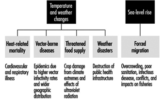 Humans have an enormous capacity to adapt to climatic and environmental conditions. However, the rate of predicted climatic and potential ecological change is of great concern to medical and earth scientists alike. Many of the health effects will be mediated through ecological responses to altered climate conditions. For example, spread of vector-borne diseases will depend on shifts in vegetation and availability of reservoir or intermediate hosts, in conjunction with the direct effects of temperature and humidity on parasites and their vectors (Patz et al. 1996). Understanding the hazards of climate change will, therefore, require an integrated ecological risk assessment which demands new and complex approaches compared to conventional single-agent cause-and-effect risk analysis from empirical data (McMichael 1993).

Stratospheric Ozone Depletion

Stratospheric ozone depletion is occurring primarily from reactions with halogen free radicals from chlorofluorocarbons (CFCs), along with other halocarbons and methyl bromide (Molina and Rowland 1974). Ozone specifically blocks the penetration of ultravioletB radiation (UVB), which contains the most biologically destructive wavelengths (290-320 nanometres). UVB levels are expected to rise disproportionately in temperate and arctic zones, since a clear relationship has been established between higher latitudes and the extent of ozone thinning (Stolarski et al. 1992).

For the period 1979-91, average ozone loss has been estimated at 2.7% per decade, correcting for solar cycle and other factors (Gleason et al. 1993). In 1993, researchers using a sensitive new spectroradiometer in Toronto, Canada, discovered that current ozone depletion has caused local increases in ambient UVB radiation of 35% in winter and 7% in summer, relative to 1989 levels (Kerr and McElroy 1993). Earlier estimates by the UN Environment Programme (UNEP) predicted a 1.4% rise in UVB per 1% drop in stratospheric ozone (UNEP 1991a).

The direct health impacts from stratospheric ozone depletion, which leads to increased ambient UVB radiation, include (1) skin cancer (2) ocular diseases and (3) immunosuppression. Indirect effects to health may occur from crop damage by ultraviolet radiation.

Health Effects of Temperature and Precipitation Change

Heat-related morbidity and mortality

Physiologically, humans have a great capacity for thermoregulation up to a threshold temperature. Weather conditions exceeding threshold temperatures and persisting for several consecutive days cause increased mortality in the population. In large cities, poor housing combined with the urban “heat island” effect further exacerbate conditions. In Shanghai, for instance, this effect can be as high as 6.5 °C on a windless evening during winter (IPCC 1990). Most heat-related fatalities occur in the elderly population and are attributed to cardiovascular and respiratory disorders (Kilbourne 1989). Key meteorological variables contribute to heat-related mortality, the most significant being high night-time readings; the greenhouse effect is predicted to especially elevate these minimum temperatures (Kalkstein and Smoyer 1993).

Temperate and polar regions are expected to warm disproportionately more than tropical and subtropical zones (IPCC 1990). Based on predictions by the US National Aeronautics and Space Administration (NASA), average summer temperatures in New York and St. Louis, for example, would rise by 3.1 and 3.9 °C, respectively, if ambient CO₂ doubles. Even with adjustment for physiological acclimatization, annual summer mortality in temperate cities such as these could rise over fourfold (Kalkstein and Smoyer 1993).

Atmospheric chemistry is an important contributing factor in the formation of urban photochemical smog, whereby photodecomposition of NO₂ in the presence of volatile organic compounds results in the production of tropospheric (ground-level) ozone. Both increased ambient UV radiation and warmer temperatures would further drive these reactions. Adverse health effects from air pollution are well known, and continued fossil fuel use will extend acute and chronic health impacts. (see “Air pollution” in this chapter).

Infectious diseases and climate/ecosystem change

Coupled atmosphere-ocean general circulation models predict that high latitudes in the northern hemisphere will experience the largest surface temperature elevation based on current IPCC scenarios (IPCC 1992). Minimum winter temperatures are expected to be disproportionately more affected, allowing for certain viruses and parasites to extend into regions where they previously could not live. In addition to direct climate effects on vectors, transformation of ecosystems could have marked implications for diseases whereby the geographic range of vector and/or reservoir host species is defined by these ecosystems.

Vector-borne diseases may spread to temperate regions in both hemispheres and intensify in endemic areas. Temperature determines vector infectivity by affecting pathogen replication, maturation and the period of infectivity (Longstreth and Wiseman 1989). Elevated temperature and humidity also intensify the biting behaviour of several mosquito species. Extreme heat, on the other hand, can shorten insect survival time.

Infectious diseases which incorporate a cold-blooded species (invertebrate) within their life cycles, are most susceptible to subtle climate variations (Sharp 1994). Diseases whose infectious agents, vectors or hosts are affected by climate change include malaria, schistosomiasis, filariasis, leishmaniasis, onchocerciasis (river blindness), trypanosomiasis (Chagas’ and African sleeping sickness), dengue, yellow fever and arboviral encephalitis. Current figures of the number of people at risk of these diseases are listed in table 1 (WHO 1990d).

Table 1. Global status of major vector-borne diseases

^a The numbers refer to explanations in the text. ^b Based on a world population estimated at 4.8 billion (1989).
0 = unlikely; + = likely; ++ = very likely; +++ = no estimate available; ? = not known.

Worldwide, malaria is the most prevalent vector-borne disease and causes one to two million deaths annually. An estimated one million additional annual fatalities may arise from climate change by the middle of the next century, according to Martens et al. (1995). The Anopheline mosquito which carries malaria can extend to the 16 °C winter isotherm, since parasite development does not occur below this temperature (Gilles and Warrell 1993). Epidemics occurring at higher altitudes generally coincide with above average temperatures (Loevinsohn 1994). Deforestation also affects malaria, since cleared areas provide an abundance of freshwater pools in which Anopheline larvae can develop (see “Species extinction, biodiversity loss and human health” in this chapter).

Over the past two decades, efforts to control malaria have made only marginal gains. Treatment has not improved as drug-resistance has become a major problem for the most virulent strain, Plasmodium falciparum, and antimalarial vaccines have shown only limited efficacy (Institute of Medicine 1991). Great capacity for antigenic variation of protozoans has thus far prevented acquisition of effective vaccines for malaria and sleeping sickness, leaving little optimism for readily available new pharmaceutical agents against these diseases. Diseases which involve intermediate reservoir hosts (e.g., deer and rodents in the case of Lyme disease) make human herd immunity from vaccination programmes essentially unattainable, representing another hurdle to preventive medical intervention.

As climate change alters habitat, causing a potential reduction of biodiversity, insect vectors will be forced to find new hosts (see “Species extinction, biodiversity loss and human health”). In Honduras, for example, blood-seeking insects such as the assassin beetle, which carries incurable Chagas’ disease (or American Trypanosomiasis), has been forced to seek human hosts as biodiversity decreases from deforestation. Of 10,601 Hondurans studied in endemic regions, 23.5% are now seropositive for Chagas’ disease (Sharp 1994). Zoonotic diseases are frequently the source of human infections, and generally affect man after an environmental change or alteration of human activity (Institute of Medicine l992). Many “newly emerging” diseases in humans are actually long-standing zoonoses of animal host species. For example, Hantavirus, recently found to be the cause of human fatalities in the southwest United States, has long been established in rodents and the recent outbreak was felt to be related to climatic/ecological conditions (Wenzel 1994).

Marine effects

Climate change may further impact public health through effects on harmful marine phytoplankton (or algae) blooms. Increases in phytoplankton globally has been a consequence of poor erosion control management, liberal agricultural application of fertilizers, and coastal sewage release, all resulting in effluents rich in nutrients which promote algae growth. Conditions that favour this growth could be augmented by warmer sea surface temperatures expected with global warming. Overharvesting of fish and shellfish (algae consumers) coupled with widespread pesticide use toxic to fish, further contribute to plankton overgrowth (Epstein 1995).

Red tides causing diarrhoeal and paralytic diseases and amnesic shellfish poisoning are prime examples of diseases stemming from algal overgrowth. Vibrio cholera has been found to be harboured by marine phytoplankton; thus blooms could represent an expanded reservoir from which cholera epidemics may initiate (Huq et al. 1990).

Food supply and human nutrition

Malnutrition is a major cause of infant mortality and childhood morbidity due to immunosuppression (see “Food and agriculture”). Climate change could adversely affect agriculture both by long-term changes, such as reducing soil moisture through evapotranspiration, and, more immediately, by extreme weather events such as droughts, flooding (and erosion) and tropical storms. Plants may initially benefit from “CO₂ fertilization”, which can enhance photosynthesis (IPCC 1990). Even accounting for this, agriculture in developing countries will suffer most, and it is estimated that in these nations, 40-300 million additional people will be at risk from hunger due to climate change (Sharp 1994).

Indirect ecological changes affecting crops will need to be considered as well, since agricultural pests may change in distribution (IPCC 1992) (see “Food and agriculture”). Considering complex ecosystem dynamics, complete assessment will need to extend beyond the direct impacts of changing atmospheric and/or soil conditions.

Health Effects of Weather Disasters and Sea Level Rise

Thermal expansion of oceans may cause sea level to rise at a relatively rapid rate of two to four centimetres per decade, and projected extremes of the hydrologic cycle are expected to produce more severe weather patterns and storms. Such events would directly disrupt dwellings and public health infrastructures, such as sanitation systems and stormwater drainage (IPCC 1992). Vulnerable populations in low-lying coastal areas and small islands would be forced to migrate to safer locations. Resulting overcrowding and poor sanitation among these environmental refugees could amplify the spread of infectious diseases such as cholera, and vector-borne disease transmission rates would escalate due to crowding and potential influxes of infected individuals (WHO 1990d). Flooded drainage systems may further exacerbate the situation, and psychological impacts must also be considered from post-traumatic stress syndrome following major storms.

Fresh water supply would diminish due to saline intrusion of coastal aquifers and coastal farmland lost to salination or outright inundation. For example, a sea-level rise of one metre would destroy 15% and 20% of agriculture in Egypt and Bangladesh respectively (IPCC 1990). As for droughts, adaptive irrigation methods could affect arthropod and invertebrate breeding sites of vectors (e.g., similar to schistosomiasis in Egypt), but cost/benefit evaluation of such impacts will be difficult.

Health Effects of Stratospheric Ozone Depletion

Direct health effects of ultravioletB radiation

Ozone specifically blocks the penetration of ultravioletB radiation, which contains the most biologically destructive wavelengths of 290-320 nanometres. UVB induces the formation of pyrimidine dimers within DNA molecules, which if unrepaired can evolve to cancer (IARC 1992). Non-melanoma skin cancer (squamous and basal cell carcinoma) and superficial spreading melanoma are correlated with sunlight exposure. In Western populations, melanoma incidence has increased by 20 to 50% every five years over the past two decades (Coleman et al. 1993). While there is no direct relationship between cumulative ultraviolet exposure and melanoma, excessive UV exposure during childhood is associated with incidence. For a sustained 10% decline in the stratospheric ozone layer, non-melanoma skin cancer cases could rise by 26%, or 300,000 globally per year; melanoma could increase by 20%, or 4,500 more cases annually (UNEP 1991a).

Eye cataract formation causes half of the world’s blindness (17 million cases annually) and is associated with UVB radiation in a dose-response relationship (Taylor 1990). Amino acids and membrane transport systems in the lens of the eye are especially prone to photo oxidation by oxygen radicals generated by UVB irradiation (IARC 1992). A doubling of UVB exposure could cause a 60% increase in cortical cataracts over current levels (Taylor et al. 1988). UNEP estimates that a 10% sustained loss of stratospheric ozone would result in nearly 1.75 million extra cataracts annually (UNEP 1991a). Other ocular effects of UVB exposure include photokeratitis, photokerato-conjunctivitis, pinguecula and pterygium (or overgrowth of the conjunctival epithelium) and climatic droplet keratopathy (IARC 1992).

The ability of the immune system to function effectively depends on “local” antigen processing and presentation to T-cells, as well as augmentation of the “systemic” response via lymphokine (biochemical messenger) production and resultant T-helper/T-suppressor cell ratios. UVB causes immunosuppression at both levels. UVB in animal studies can affect the course of infectious skin diseases, such as onchocerciasis, leishmaniasis and dermatophytosis, and impair immunosurveillance of transformed, precancerous epidermal cells. Preliminary studies further show an influence on vaccine efficacy (Kripke and Morison 1986; IARC 1992).

Indirect public health effects of UVB

Historically, terrestrial plants became established only after the formation of the shielding ozone layer, since UVB inhibits photosynthesis (UNEP 1991a). Weakening of food crops susceptible to UVB damage could further extend the impacts on agriculture due to climate changes and sea-level rise.

Phytoplankton are at the foundation of the marine food chain and also serve as an important carbon dioxide “sink”. UV damage to these algae in polar regions, therefore, would detrimentally affect the marine food chain and exacerbate the greenhouse effect. UNEP estimates that a 10% loss of marine phytoplankton would limit the oceans’ annual CO₂ uptake by five gigatonnes, which equals the yearly anthropogenic emissions from fossil fuel combustion (UNEP 1991a).

Occupational Hazards and Control Strategies

Occupational hazards

With regard to reduction in GHG emissions from fossil fuels, alternate renewable energy sources will need to be expanded. The public and occupational hazards of nuclear energy are well known, and safeguarding plants, workers and spent fuel will be necessary. Methanol may serve to replace much gasoline usage; however, formaldehyde emission from these sources will present a new environmental hazard. Superconducting materials for energy efficient electricity transfer are mostly ceramics comprised of calcium, strontium, barium, bismuth, thallium and yttrium (WHO in press).

Less is known about the occupational safety in the manufacturing units for solar energy capture. Silicon, gallium, indium, thallium, arsenic and antimony are the primary elements used to build photovoltaic cells (WHO in press). Silicon and arsenic adversely affect the lungs; gallium is concentrated in the kidney, liver, and bone; and ionic forms of indium are nephrotoxic.

The destructive effects of CFCs on the stratospheric ozone layer were recognized in the 1970s, and the US EPA banned these inert propellants in aerosols in 1978. By 1985, widespread concern erupted when an Antarctic-based British team discovered the “hole” in the ozone layer (Farman, Gardiner and Shanklin 1985). Subsequent passage of the Montreal Protocol in 1987, with amendments in 1990 and 1992, has already mandated sharp cuts in CFC production.

The replacement chemicals for CFCs are the hydrochlorofluorocarbons (HCFCs) and the hydrofluorocarbons (HFCs). The presence of the hydrogen atom may more readily subject these compounds to degradation by hydroxyl radicals (OH^–) in the troposphere, thus reducing potential stratospheric ozone depletion. These CFC replacement chemicals are, however, more biologically reactive than CFCs. The nature of a C-H bond makes these chemicals prone to oxidation via the cytochrome P-450 system (WHO in press).

Mitigation and adaptation

Meeting the public health challenges presented by global climate change will require (1) an integrated ecological approach; (2) reduction of greenhouse gases through industrial emission control, land use policies to maximize the extent of CO₂ “sinks” and population policies to achieve both; (3) monitoring of biological indicators on both regional and global scales; (4) adaptive public health strategies to minimize the impacts from unavoidable climate change; and (5) cooperation between developed and developing nations. In short, increased integration of environmental and public health policies must be promoted.

Climate change and ozone depletion present a vast number of health risks at multiple levels and underscore the important relationship between ecosystem dynamics and sustained human health. Preventive measures must therefore be systems based, and must anticipate significant ecological responses to climate change as well as the direct physical hazards predicted. Some key elements to consider in an ecological risk assessment will include spatial and temporal variations, feedback mechanisms and use of lower level organisms as early biological indicators.

Reduction of greenhouse gases by diverting from fossil fuels to renewable energy resources represents primary prevention of climate change. Similarly, strategic land use planning and stabilization of population stress on the environment will preserve important natural greenhouse gas sinks.

Because some climate change may be unavoidable, secondary prevention through early detection by monitoring of health parameters will require unprecedented coordination. For the first time in history, attempts are being made to monitor the earth system in its entirety. The Global Climate Observing System incorporates the World Weather Watch and Global Atmosphere Watch of the World Meteorological Organization (WMO) with parts of UNEP’s Global Environmental Monitoring System. The Global Ocean Observing System is a new joint endeavour by the Intergovernmental Oceanographic Commission of UN Educational, Scientific and Cultural Organization (UNESCO), WMO and the International Council of Scientific Unions (ICSU). Both satellite and underwater measurements will be utilized to monitor changes in marine systems. The Global Terrestrial Observing System is a new system sponsored by UNEP, UNESCO, WMO, ICSU and the Food and Agricultural Organization (FAO), and will provide the terrestrial component of the Global Climate Observing System (WMO 1992).

Adaptive options to reduce unavoidable health consequences include disaster preparedness programmes; urban planning to reduce the “heat island” effect and improve housing; land use planning to minimize erosion, flash flooding and unnecessary deforestation (e.g., halting the creation of rangeland for meat exportation); personal adaptive behaviours, such as avoiding sun exposure; and vector-control and expanded vaccination efforts. Unintended costs of adaptive control measures of, for example, increased pesticide use will require consideration. Over-dependence on pesticides not only leads to insect resistance but also eliminates natural, beneficial, predatory organisms. The adverse effect on public health and the environment due to current pesticide use is estimated to be between US$100 billion and US$200 billion annually (Institute of Medicine 1991).

Developing countries will suffer disproportionately more from the consequences of climate change, though industrialized nations are presently more responsible for GHGs in the atmosphere. In the future poorer countries will influence the course of global warming significantly more, both through the technologies they choose to adopt as their development accelerates, and by land use practices. Developed nations will need to embrace more environmentally sound energy policies and promptly transfer new (and affordable) technology to developing countries.

Case Study: Mosquito-borne viruses

Mosquito-borne encephalitis and dengue fever are prime examples of vector-borne diseases whose distributions are limited by climate. Epidemics of St. Louis encephalitis (SLE), the most common arboviral encephalitis in the United States, generally occur south of the 22°C June isotherm, but northerly outbreaks have occurred during unseasonably warm years. Human outbreaks are highly correlated with several-day periods when temperature exceeds 27°C (Shope 1990).

Field studies on SLE indicate that a 1°C increase in temperature significantly shortens the elapsed time between a mosquito blood-meal and viral replication to the point of infectivity within the vector, or the extrinsic incubation period. Adjusting for reduced adult mosquito survival at elevated temperatures, a 3 to 5 °C temperature increase is predicted to cause a significant northern shift of SLE outbreaks (Reeves et al. 1994).

The range of the primary mosquito vector of dengue (and yellow fever), Aedes aegypti, extends to 35° latitude because freezing temperatures kill both larvae and adults. Dengue is widespread in the Caribbean, tropical America, Oceania, Asia, Africa and Australia. Over the past 15 years, dengue epidemics have increased in both numbers and severity, especially in tropical urban centres. Dengue haemorrhagic fever now ranks as one of the leading causes for hospitalization and mortality of children in Southeast Asia (Institute of Medicine 1992). The same increasing pattern observed in Asia 20 years ago is now occurring in the Americas.

Climate change can potentially alter dengue transmission. In Mexico in 1986, the most important predictor of dengue transmission was found to be the median temperature during the rainy season, with an adjusted fourfold risk observed between 17 °C and 30 °C (Koopman et al. 1991). Lab studies support these field data. In vitro, the extrinsic incubation period for dengue type-2 virus was 12 days at 30 °C and only seven days at 32 to 35 °C (Watts et al. 1987). This temperature effect of shortening the incubation period by five days translates to a potentially threefold higher transmission rate of disease (Koopman et al. 1991). Finally, warmer temperatures result in the hatching of smaller adults, which must bite more frequently to develop an egg batch. In summary, increased temperatures can lead to more infectious mosquitoes that bite more frequently (Focks et al. 1995).

Back

Urbanization is a major feature of the contemporary world. At the beginning of the nineteenth century there were some 50 million people living in urban areas. By 1975 there were 1.6 billion, and by the year 2000 there will be 3.1 billion (Harpham, Lusty and Vaugham 1988). Such figures outstrip by far the growth of rural population.

However, the process of urbanization has often had hazardous impacts on the health of those who work and live in cities and towns. To a greater or lesser extent, the production of adequate housing, the provision of urban infrastructure and the control of traffic has not kept pace with the growth of urban population. This has generated a myriad of health problems.

Housing

Housing conditions throughout the world are far from adequate. For example, by the mid-1980s, 40 to 50% of the population in many cities in developing countries were living in substandard accommodations (WHO Commission on Health and Environment 1992b). Such figures have increased ever since. Although the situation in industrialized countries is less critical, housing problems such as decay, overcrowding and even homelessness are frequent.

The major aspects of the residential environment which influence health, and their associated hazards, are presented in table 1. The health of a worker is likely to be affected if his or her residence is deficient in one or more of these aspects. In developing countries, for instance, some 600 million urban dwellers live in health- and life-threatening homes and neighbourhoods (Hardoy, Cairncross and Satterthwaite 1990; WHO 1992b).

Table 1. Housing and health

Source: Hardoy et al. 1990; Harpham et al. 1988; WHO Commission on Health and Environment 1992b.

Housing problems may also have a direct effect on occupational health, in the case of those who work in residential environments. Those include domestic servants and also a growing number of small-scale producers in a variety of cottage industries. These producers may be further affected when their production processes generate some form of pollution. Selected studies in these types of industries have detected hazardous wastes with consequences such as cardiovascular diseases, skin cancer, neurological disorders, bronchial cancer, photophobia and infant methaemoglobinaemia (Hamza 1991).

Prevention of home-related problems includes action in different stages of housing provision:

1. location (e.g., safe and vector-free sites)
2. house design (e.g., spaces with adequate size and climatic protection, use of non-perishable building materials, adequate protection for equipment)
3. construction (prevention of construction defects)
4. maintenance (e.g., proper control of equipment, proper screening).

The insertion of industrial activities in the residential environment may require special measures of protection, according to the particular process of production.

The specific housing solutions may vary widely from place to place, depending on the social, economic, technical and cultural circumstances. A great number of cities and towns do have local planning and building legislation that includes measures to prevent health hazards. However, such legislation is often not enforced due to ignorance, lack of legal control or, in most cases, lack of financial resources to build proper housing. Therefore, it is important not only to design (and update) adequate codes, but also to create the conditions for their implementation.

Urban Infrastructure: The Provision of Environmental Health Services

Housing may also affect health when it is not properly supplied with environmental health services such as garbage collection, water, sanitation and drainage. The inadequate provision of these services, however, extend beyond the housing realm, and may cause hazards for the city or town as a whole. Standards of provision of these services are still critical in a large number of places. For example, 30 to 50% of solid waste generated within urban centres is left uncollected. In 1985 there were 100 million more people without water service than in 1975. More than two billion people still have no sanitary means to dispose of human waste (Hardoy, Cairncross and Satterthwaite 1990; WHO Commission on Health and Environment 1992b). And the media have frequently shown cases of floods and other accidents connected to inadequate urban drainage.

Hazards derived from deficient provision of environmental health services are presented in table 2. Cross-service hazards are also common—e.g., contamination of water supply due to lack of sanitation, dissemination of refuse through non-drained water. To give one illustration of the extent of infrastructural problems among many, a child is killed worldwide every 20 seconds due to diarrhoea—which is a major outcome of deficient environmental health services.

Table 2. Urban infrastructure and health

Source: Hardoy et al. 1990; WHO Commission on Health and Environment 1992b.

Those labourers whose immediate or wider working environment is not adequately supplied with such services are exposed to a profusion of occupational health risks. Those who work in the provision or maintenance of services, such as garbage pickers, sweepers and scavengers, are further exposed.

There exist indeed technical solutions capable of ameliorating the provision of environmental health services. They encompass, among many others, garbage recycling schemes (including support to scavengers), use of different kinds of garbage collection vehicles to reach different types of roads (including those of informal settlements), water-saving fittings, tighter control of water leakages and low-cost sanitation schemes such as ventilated pit latrines, septic tanks or small-bore sewers.

However, the success of each solution will depend on its appropriateness to the local circumstances and on the local resources and capacity to implement it. Political willingness is fundamental, but not enough. Governments have frequently found it difficult to provide urban services adequately by themselves. Success stories of good supply have often included cooperation between the public, private and/or voluntary sectors. A thorough involvement and support of the local communities is important. This often requires official recognition of the large number of illegal and semi-legal settlements (especially but not only in developing countries), which bear a heavy part of the environmental health problems. Workers directly involved in services such as garbage collection or recycling and sewerage maintenance need special equipment for protection, such as gloves, overalls and masks.

Traffic

Cities and towns have depended heavily on ground transport for the movement of people and goods. Thus, the increase in urbanization throughout the world has been accompanied by a sharp growth in urban traffic. However, such a situation has generated a large number of accidents. Some 500,000 people are killed in traffic accidents each year, two-thirds of which occur in urban or peri-urban areas. In addition, according to many studies in different countries, for every death there are ten to twenty persons injured. Many cases suffer permanent or prolonged loss of productivity (Urban Edge 1990a; WHO Commission on Health and Environment 1992a). A large share of such data relates to people on their way to or from work—and such a type of traffic accident has lately been considered an occupational hazard.

According to World Bank studies, the main causes of urban traffic accidents include: poor condition of vehicles; deteriorated streets; different types of traffic—from pedestrians and animals to trucks—sharing the same streets or lanes; non-existent foot-paths; and reckless road behaviour (both from drivers and pedestrians) (Urban Edge 1990a, 1990b).

A further hazard generated by the expansion of urban traffic is air and noise pollution. Health problems include acute and chronic respiratory diseases, malignancies and hearing deficiencies (pollution is also dealt with in other articles in this Encyclopaedia).

Technical solutions to ameliorate road and car safety (as well as pollution) abound. The major challenge seems to be changing the attitudes of drivers, pedestrians and public officials. Road safety education—from elementary school teaching to campaigns throughout the media—has often been recommended as a policy to target drivers and/or pedestrians (and such programmes have often had some degree of success when implemented). Public officials have the responsibility to design and enforce traffic legislation, inspect vehicles and design and implement engineering safety measures. However, according to the aforementioned studies, these officials seldom perceive traffic accidents (or pollution) as a top priority, or have the means to act dutifully (Urban Edge 1990a, 1990b). Therefore, they have to be targeted by educational campaigns, and supported in their work.

The Urban Fabric

In addition to the specific issues already noted (housing, services, traffic), the overall growth of the urban fabric also has had an impact on health. Firstly, urban areas are usually dense, a fact which facilitates the spread of communicable diseases. Secondly, such areas concentrate a large number of industries, and their associated pollution. Thirdly, through the process of urban growth, natural foci of disease vectors may get entrapped within new urban areas, and new niches for disease vectors may be established. Vectors may adapt to new (urban) habitats—for example, those responsible for urban malaria, dengue and yellow fever. Fourthly, urbanization has often had psychosocial consequences such as stress, alienation, instability and insecurity; which, in their turn, have led to problems such as depression and alcohol and drug abuse (Harpham, Lusty and Vaugham 1988; WHO Commission on Health and Environment 1992a).

Past experiences have demonstrated the possibility (and the need) to tackle health problems via improvements in urbanization. For instance, “¼ the remarkable decline in mortality rates and improvements in health in Europe and North America at the turn of the last century owe more to improved nutrition and improvements in water supply, sanitation and other aspects of housing and living conditions than to medical establishments” (Hardoy, Cairncross and Satterthwaite 1990).

Solutions for the mounting problems of urbanization need sound integration between (often separated) urban planning and management, and the participation of the different public, private and voluntary actors which operate in the urban arena. Urbanization affects a wide range of workers. Contrary to other sources or types of health problems (which might affect specific categories of workers), occupational hazards derived from urbanization cannot be dealt with through single trade union action or pressure. They require inter-profession action, or, even more broadly, action from the urban community in general.

Back

The WHO Commission on Health and Environment (1992a) Panel on Energy considered four energy-related issues to be of the highest immediate and/or future concern for environmental health:

1. exposure to noxious agents in the course of domestic utilization of biomass and coal
2. exposure resulting from urban air pollution in numerous large cities of the world
3. the possible health-related impacts of climate change
4. serious accidents with environmental impacts on the health of the general public.

Quantitative assessment of the health risks from different energy systems requires system-wide evaluation of all steps in a fuel cycle, starting with extraction of raw resources, and concluding with the final consumption of energy. For valid intertechnology comparisons to be made, methods, data and end-use demands must be similar and specified. In quantifying the effects of end-use demands, differences in conversion efficiencies of energy- and fuel-specific devices to useful energy must be evaluated.

Comparative assessment is built around the idea of the Reference Energy System (RES), which depicts fuel cycles step-by-step, from extraction through processing to combustion and ultimate disposal of wastes. The RES provides a common, simple framework for defining flows of energy and related data used for risk assessment. An RES (figure 1) is a network representation of the main components of an energy system for a given year, specifying resource consumption, fuel transportation, conversion processes and end uses, thereby compactly incorporating the salient features of the energy system while providing a framework for assessment of major resource, environmental, health and economic effects that can result from new technologies or policies.

Figure 1. Reference energy system, year 1979

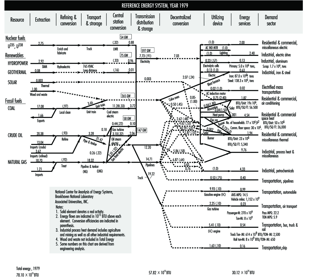
Based on their health risks, energy technologies can be classified into three groups:

1. The fuels group is characterized by use of large amounts of fossil fuels or biomass—coal, oil, natural gas, wood and so on—the collection, processing and transport of which have high accident rates that dominate occupational risks and the burning of which produces large amounts of air pollution and solid waste that dominate public risks.
2. The renewable group is characterized by use of diffuse renewable resources with low energy density—sun, wind, water—which are available in enormous quantities at no cost, but the capturing of which requires large areas and construction of expensive facilities capable of “concentrating” them into useful forms. Occupational risks are high and dominated by construction of the facilities. Public risks are low, mostly confined to low-probability accidents, such as dam failures, equipment failures and fires.
3. The nuclear group includes nuclear fission technologies, distinguished by extremely high energy densities in the processed fuel, with corresponding low quantities of fuel and wastes to process, but with low concentrations in the earth’s crust, necessitating a large mining or collection effort. Occupational risks are, therefore, relatively high and dominated by mining and processing accidents. Public risks are small and dominated by routine operations of reactors. Special attention must be given to public fears of risks from exposure to radiation from nuclear technologies—fears which are relatively large per unit risk to health.

The significant health effects of technologies for generating electricity are shown in table 1, table 2 and table 3.

Table 1. Significant health effects of technologies for generating electricity - fuels group

* As an energy source, usually considered as renewable.

Table 2. Significant health effects of technologies for generating electricity - renewable group

Table 3. Significant health effects of technologies for generating electricity - nuclear group

Studies of health effects of wood burning in the United States, like analyses of other energy sources, were based on the health effects of supplying a unit amount of energy, that is, that needed to heat one million dwelling years. This is 6 ×10⁷ GJ heat, or 8.8 ×10⁷ GJ wood input at 69% efficiency. Health effects were estimated in gathering, transport and combustion stages. Oil and coal alternatives were scaled from earlier work (see figure 2). The uncertainties in gathering are ± a factor of ~2, those in home fires ± a factor of ~3, and those in air pollution ± a factor greater than 10. If the hazards of nuclear electric were plotted on the same scale, the total risk would be approximately one-half that of mining for coal mining.

Figure 2. Health effects per unit amount of energy

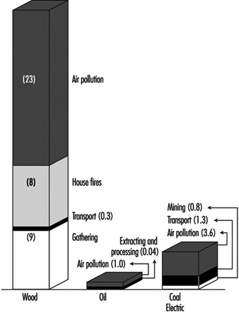
A convenient way to help understand the risk is to scale it to a single person supplying one dwelling with wood over 40 years (figure 3). This results in a total risk of fatality of ~1.6 x 10^–3 (i.e., ~0.2%). This can be compared with the risk of death in an automobile accident in the United States during the same time, ~9.3 x 10^–3 (i.e., ~1%), which is five times greater. Wood burning presents risks which are of the same order as more conventional heating technologies. Both are well below the overall risk of other common activities, and many aspects of the risk are clearly amenable to preventive measures.

Figure 3. Risk, to a single person, of fatality due to supplying one dwelling with wood fuel for 40 years

The following comparisons for health risks can be made:

• Acute occupational risk. For the coal cycle, occupational risk is distinctly higher than that associated with oil and gas; it is about the same as that associated with renewable energy systems, when their construction is included in the assessment, and it is about 8-10 times higher than the corresponding risks for nuclear. Future technological advances in renewable solar and wind energy sources may result in a significant reduction in the acute occupational risk associated with these systems. Hydro-electricity generation entails comparatively high acute occupational risk.
• Late occupational risk. Late fatalities arise mainly in coal and uranium mining, and are roughly of the same size. Underground coal mining, however, appears to be more dangerous than underground uranium mining (calculation from the basis of a normalized unit of electricity generated). Use of surface-mined coal, on the other hand, leads in total to fewer late fatalities than does use of nuclear energy.
• Acute public risk. These risks, mostly due to transportation accidents, are highly dependent on distance travelled and mode of transport. The risk of nuclear is 10-100 times lower than those of all the other options, mainly because of the relatively low quantity of materials to be transported. The coal cycle has the highest acute public risk because of the large material transport using the same reasoning.
• Late public risk. There are great uncertainties associated with late public risks associated with all the energy sources. Late public risks for nuclear and natural gas are about equal and are, at least ten times lower than those associated with coal and oil. Future developments are expected to result in significant decreases in late public risks for renewables.

Clearly, health effects of different energy sources depend on the quantity and type of energy use. These vary greatly geographically. Fuelwood is the fourth largest contribution to world energy supply, after petroleum, coal and natural gas. Close to half the world population, especially those living in the rural and urban areas of developing countries, depend on it for cooking and heating (either wood or its derivative, charcoal, or, in the absence of either of these, on agricultural residues or dung). Fuelwood constitutes more than half the world’s consumption of wood, rising to 86% in developing countries and 91% in Africa.

In considering new and renewable sources of energy such as solar energy, wind power, and alcohol fuels, the idea of a “fuel cycle” must encompass industries such as solar photovoltaics, where virtually no risk attaches to the operation of the device but a substantial amount—often ignored—may be involved in its manufacture.

Attempts were made to deal with this difficulty by expanding the fuel cycle concept to include all stages in developing an energy system—including, for example, the concrete that goes into the plant that manufactures the glass for the solar collector. The issue of completeness has been addressed by noting that the backward analysis of manufacturing steps is equivalent to a set of simultaneous equations whose solution—if linear—is expressible as a matrix of values. Such an approach is familiar to economists as input-output analysis; and the appropriate numbers, showing how much each economic activity draws on the others, have already been derived—although for aggregate categories that may not exactly match the manufacturing steps one wishes to scrutinize for measuring health damage.

No single method of comparative risk analysis in the energy industry is fully satisfactory by itself. Each has advantages and limitations; each provides a different kind of information. Given the level of uncertainty of health risk analyses, results from all methods should be examined to provide as detailed a picture as possible, and fuller understanding of the magnitudes of associated uncertainties.

Back