- You are here:
-
Home

- Part IV. Tools and Approaches

Children categories

27. Biological Monitoring (6)

27. Biological Monitoring
Chapter Editor: Robert Lauwerys
Table of Contents
Tables and Figures
General Principles
Vito Foà and Lorenzo Alessio
Quality Assurance
D. Gompertz
Metals and Organometallic Compounds
P. Hoet and Robert Lauwerys
Organic Solvents
Masayuki Ikeda
Genotoxic Chemicals
Marja Sorsa
Pesticides
Marco Maroni and Adalberto Ferioli
Tables
Click a link below to view table in article context.
1. ACGIH, DFG & other limit values for metals
2. Examples of chemicals & biological monitoring
3. Biological monitoring for organic solvents
4. Genotoxicity of chemicals evaluated by IARC
5. Biomarkers & some cell/tissue samples & genotoxicity
6. Human carcinogens, occupational exposure & cytogenetic end points
8. Exposure from production & use of pesticides
9. Acute OP toxicity at different levels of ACHE inhibition
10. Variations of ACHE & PCHE & selected health conditions
11. Cholinesterase activities of unexposed healthy people
12. Urinary alkyl phosphates & OP pesticides
13. Urinary alkyl phosphates measurements & OP
14. Urinary carbamate metabolites
15. Urinary dithiocarbamate metabolites
16. Proposed indices for biological monitoring of pesticides
17. Recommended biological limit values (as of 1996)
Figures
Point to a thumbnail to see figure caption, click to see figure in article context.
|
|


28. Epidemiology and Statistics (12)
28. Epidemiology and Statistics
Chapter Editors: Franco Merletti, Colin L. Soskolne and Paolo Vineis
Table of Contents
Tables and Figures
Epidemiological Method Applied to Occupational Health and Safety
Franco Merletti, Colin L. Soskolne and Paolo Vineis
Exposure Assessment
M. Gerald Ott
Summary Worklife Exposure Measures
Colin L. Soskolne
Measuring Effects of Exposures
Shelia Hoar Zahm
Case Study: Measures
Franco Merletti, Colin L. Soskolne and Paola Vineis
Options in Study Design
Sven Hernberg
Validity Issues in Study Design
Annie J. Sasco
Impact of Random Measurement Error
Paolo Vineis and Colin L. Soskolne
Statistical Methods
Annibale Biggeri and Mario Braga
Causality Assessment and Ethics in Epidemiological Research
Paolo Vineis
Case Studies Illustrating Methodological Issues in the Surveillance of Occupational Diseases
Jung-Der Wang
Questionnaires in Epidemiological Research
Steven D. Stellman and Colin L. Soskolne
Asbestos Historical Perspective
Lawrence Garfinkel
Tables
Click a link below to view table in article context.
1. Five selected summary measures of worklife exposure
2. Measures of disease occurrence
3. Measures of association for a cohort study
4. Measures of association for case-control studies
5. General frequency table layout for cohort data
6. Sample layout of case-control data
7. Layout case-control data - one control per case
8. Hypothetical cohort of 1950 individuals to T2
9. Indices of central tendency & dispersion
10. A binomial experiment & probabilities
11. Possible outcomes of a binomial experiment
12. Binomial distribution, 15 successes/30 trials
13. Binomial distribution, p = 0.25; 30 trials
14. Type II error & power; x = 12, n = 30, a = 0.05
15. Type II error & power; x = 12, n = 40, a = 0.05
16. 632 workers exposed to asbestos 20 years or longer
17. O/E number of deaths among 632 asbestos workers
Figures
Point to a thumbnail to see figure caption, click to see the figure in article context.
|
|


29. Ergonomics (27)
29. Ergonomics
Chapter Editors: Wolfgang Laurig and Joachim Vedder
Table of Contents
Tables and Figures
Overview
Wolfgang Laurig and Joachim Vedder
Goals, Principles and Methods
The Nature and Aims of Ergonomics
William T. Singleton
Analysis of Activities, Tasks and Work Systems
Véronique De Keyser
Ergonomics and Standardization
Friedhelm Nachreiner
Checklists
Pranab Kumar Nag
Physical and Physiological Aspects
Anthropometry
Melchiorre Masali
Muscular Work
Juhani Smolander and Veikko Louhevaara
Postures at Work
Ilkka Kuorinka
Biomechanics
Frank Darby
General Fatigue
Étienne Grandjean
Fatigue and Recovery
Rolf Helbig and Walter Rohmert
Psychological Aspects
Mental Workload
Winfried Hacker
Vigilance
Herbert Heuer
Mental Fatigue
Peter Richter
Organizational Aspects of Work
Work Organization
Eberhard Ulich and Gudela Grote
Sleep Deprivation
Kazutaka Kogi
Work Systems Design
Workstations
Roland Kadefors
Tools
T.M. Fraser
Controls, Indicators and Panels
Karl H. E. Kroemer
Information Processing and Design
Andries F. Sanders
Designing for Everyone
Designing for Specific Groups
Joke H. Grady-van den Nieuwboer
Case Study: The International Classification of Functional Limitation in People
Cultural Differences
Houshang Shahnavaz
Elderly Workers
Antoine Laville and Serge Volkoff
Workers with Special Needs
Joke H. Grady-van den Nieuwboer
Diversity and Importance of Ergonomics--Two Examples
System Design in Diamond Manufacturing
Issachar Gilad
Disregarding Ergonomic Design Principles: Chernobyl
Vladimir M. Munipov
Tables
Click a link below to view table in article context.
1. Basic anthropometric core list
2. Fatigue & recovery dependent on activity levels
3. Rules of combination effects of two stress factors on strain
4. Differenting among several negative consequences of mental strain
5. Work-oriented principles for production structuring
6. Participation in organizational context
7. User participation in the technology process
8. Irregular working hours & sleep deprivation
9. Aspects of advance, anchor & retard sleeps
10. Control movements & expected effects
11. Control-effect relations of common hand controls
12. Rules for arrangement of controls
Figures
Point to a thumbnail to see figure caption, click to see the figure in the article context.


30. Occupational Hygiene (6)
30. Occupational Hygiene
Chapter Editor: Robert F. Herrick
Table of Contents
Tables and Figures
Goals, Definitions and General Information
Berenice I. Ferrari Goelzer
Recognition of Hazards
Linnéa Lillienberg
Evaluation of the Work Environment
Lori A. Todd
Occupational Hygiene: Control of Exposures Through Intervention
James Stewart
The Biological Basis for Exposure Assessment
Dick Heederik
Occupational Exposure Limits
Dennis J. Paustenbach
Tables
1. Hazards of chemical; biological & physical agents
2. Occupational exposure limits (OELs) - various countries
Figures


31. Personal Protection (7)
31. Personal Protection
Chapter Editor: Robert F. Herrick
Table of Contents
Tables and Figures
Overview and Philosophy of Personal Protection
Robert F. Herrick
Eye and Face Protectors
Kikuzi Kimura
Foot and Leg Protection
Toyohiko Miura
Head Protection
Isabelle Balty and Alain Mayer
Hearing Protection
John R. Franks and Elliott H. Berger
Protective Clothing
S. Zack Mansdorf
Respiratory Protection
Thomas J. Nelson
Tables
Click a link below to view table in article context.
1. Transmittance requirements (ISO 4850-1979)
2. Scales of protection - gas-welding & braze-welding
3. Scales of protection - oxygen cutting
4. Scales of protection - plasma arc cutting
5. Scales of protection - electric arc welding or gouging
6. Scales of protection - plasma direct arc welding
7. Safety helmet: ISO Standard 3873-1977
8. Noise Reduction Rating of a hearing protector
9. Computing the A-weighted noise reduction
10. Examples of dermal hazard categories
11. Physical, chemical & biological performance requirements
12. Material hazards associated with particular activities
13. Assigned protection factors from ANSI Z88 2 (1992)
Figures
Point to a thumbnail to see figure caption, click to see figure in article context.


32. Record Systems and Surveillance (9)
32. Record Systems and Surveillance
Chapter Editor: Steven D. Stellman
Table of Contents
Tables and Figures
Occupational Disease Surveillance and Reporting Systems
Steven B. Markowitz
Occupational Hazard Surveillance
David H. Wegman and Steven D. Stellman
Surveillance in Developing Countries
David Koh and Kee-Seng Chia
Development and Application of an Occupational Injury and Illness Classification System
Elyce Biddle
Risk Analysis of Nonfatal Workplace Injuries and Illnesses
John W. Ruser
Case Study: Worker Protection and Statistics on Accidents and Occupational Diseases - HVBG, Germany
Martin Butz and Burkhard Hoffmann
Case Study: Wismut - A Uranium Exposure Revisited
Heinz Otten and Horst Schulz
Measurement Strategies and Techniques for Occupational Exposure Assessment in Epidemiology
Frank Bochmann and Helmut Blome
Case Study: Occupational Health Surveys in China
Tables
Click a link below to view the table in article context.
1. Angiosarcoma of the liver - world register
2. Occupational illness, US, 1986 versus 1992
3. US Deaths from pneumoconiosis & pleural mesothelioma
4. Sample list of notifiable occupational diseases
5. Illness & injury reporting code structure, US
6. Nonfatal occupational injuries & illnesses, US 1993
7. Risk of occupational injuries & illnesses
8. Relative risk for repetitive motion conditions
9. Workplace accidents, Germany, 1981-93
10. Grinders in metalworking accidents, Germany, 1984-93
11. Occupational disease, Germany, 1980-93
12. Infectious diseases, Germany, 1980-93
13. Radiation exposure in the Wismut mines
14. Occupational diseases in Wismut uranium mines 1952-90
Figures
Point to a thumbnail to see figure caption, click to see the figure in article context.


33. Toxicology (21)
33. Toxicology
Chapter Editor: Ellen K. Silbergeld
Table of Contents
Tables and Figures
Introduction
Ellen K. Silbergeld, Chapter Editor
General Principles of Toxicology
Definitions and Concepts
Bo Holmberg, Johan Hogberg and Gunnar Johanson
Toxicokinetics
Dušan Djuríc
Target Organ And Critical Effects
Marek Jakubowski
Effects Of Age, Sex And Other Factors
Spomenka Telišman
Genetic Determinants Of Toxic Response
Daniel W. Nebert and Ross A. McKinnon
Mechanisms of Toxicity
Introduction And Concepts
Philip G. Watanabe
Cellular Injury And Cellular Death
Benjamin F. Trump and Irene K. Berezesky
Genetic Toxicology
R. Rita Misra and Michael P. Waalkes
Immunotoxicology
Joseph G. Vos and Henk van Loveren
Target Organ Toxicology
Ellen K. Silbergeld
Toxicology Test Methods
Biomarkers
Philippe Grandjean
Genetic Toxicity Assessment
David M. DeMarini and James Huff
In Vitro Toxicity Testing
Joanne Zurlo
Structure Activity Relationships
Ellen K. Silbergeld
Regulatory Toxicology
Toxicology In Health And Safety Regulation
Ellen K. Silbergeld
Principles Of Hazard Identification - The Japanese Approach
Masayuki Ikeda
The United States Approach to Risk Assessment Of Reproductive Toxicants and Neurotoxic Agents
Ellen K. Silbergeld
Approaches To Hazard Identification - IARC
Harri Vainio and Julian Wilbourn
Appendix - Overall Evaluations of Carcinogenicity to Humans: IARC Monographs Volumes 1-69 (836)
Carcinogen Risk Assessment: Other Approaches
Cees A. van der Heijden
Tables
Click a link below to view table in article context.
- Examples of critical organs & critical effects
- Basic effects of possible multiple interactions of metals
- Haemoglobin adducts in workers exposed to aniline & acetanilide
- Hereditary, cancer-prone disorders & defects in DNA repair
- Examples of chemicals that exhibit genotoxicity in human cells
- Classification of tests for immune markers
- Examples of biomarkers of exposure
- Pros & cons of methods for identifying human cancer risks
- Comparison of in vitro systems for hepatotoxicity studies
- Comparison of SAR & test data: OECD/NTP analyses
- Regulation of chemical substances by laws, Japan
- Test items under the Chemical Substance Control Law, Japan
- Chemical substances & the Chemical Substances Control Law
- Selected major neurotoxicity incidents
- Examples of specialized tests to measure neurotoxicity
- Endpoints in reproductive toxicology
- Comparison of low-dose extrapolations procedures
- Frequently cited models in carcinogen risk characterization
Figures
Point to a thumbnail to see figure caption, click to see figure in article context.
|
|


Pesticides
Introduction
Human exposure to pesticides has different characteristics according to whether it occurs during industrial production or use (table 1). The formulation of commercial products (by mixing active ingredients with other coformulants) has some exposure characteristics in common with pesticide use in agriculture. In fact, since formulation is typically performed by small industries which manufacture many different products in successive operations, the workers are exposed to each of several pesticides for a short time. In public health and agriculture, the use of a variety of compounds is generally the rule, although in some specific applications (for example, cotton defoliation or malaria control programmes) a single product may be used.
Table 1. Comparison of exposure characteristics during production and use of pesticides
|
Exposure on production |
Exposure on use |
|
|
Duration of exposure |
Continuous and prolonged |
Variable and intermittent |
|
Degree of exposure |
Fairly constant |
Extremely variable |
|
Type of exposure |
To one or few compounds |
To numerous compounds either in sequence or concomitantly |
|
Skin absorption |
Easy to control |
Variable according to work procedures |
|
Ambient monitoring |
Useful |
Seldom informative |
|
Biological monitoring |
Complementary to ambient monitoring |
Very useful when available |
Source: WHO 1982a, modified.
The measurement of biological indicators of exposure is particularly useful for pesticide users where the conventional techniques of exposure assessment through ambient air monitoring are scarcely applicable. Most pesticides are lipid-soluble substances that penetrate the skin. The occurrence of percutaneous (skin) absorption makes the use of biological indicators very important in assessing the level of exposure in these circumstances.
Organophosphate Insecticides
Biological indicators of effect:
Cholinesterases are the target enzymes accounting for organophosphate (OP) toxicity to insect and mammalian species. There are two principal types of cholinesterases in the human organism: acetylcholinesterase (ACHE) and plasma cholinesterase (PCHE). OP causes toxic effects in humans through the inhibition of synaptic acetylcholinesterase in the nervous system. Acetylcholinesterase is also present in red blood cells, where its function is unknown. Plasma cholinesterase is a generic term covering an inhomogeneous group of enzymes present in glial cells, plasma, liver and some other organs. PCHE is inhibited by OPs, but its inhibition does not produce known functional derangements.
Inhibition of blood ACHE and PCHE activity is highly correlated with intensity and duration of OP exposure. Blood ACHE, being the same molecular target as that responsible for acute OP toxicity in the nervous system, is a more specific indicator than PCHE. However, sensitivity of blood ACHE and PCHE to OP inhibition varies among the individual OP compounds: at the same blood concentration, some inhibit more ACHE and others more PCHE.
A reasonable correlation exists between blood ACHE activity and the clinical signs of acute toxicity (table 2). The correlation tends to be better as the rate of inhibition is faster. When inhibition occurs slowly, as with chronic low-level exposures, the correlation with illness may be low or totally non-existent. It must be noted that blood ACHE inhibition is not predictive for chronic or delayed effects.
Table 2. Severity and prognosis of acute OP toxicity at different levels of ACHE inhibition
|
ACHE inhibition (%) |
Level of poisoning |
Clinical symptoms |
Prognosis |
|
50–60 |
Mild |
Weakness, headache, dizziness, nausea, salivation, lacrimation, miosis, moderate bronchial spasm |
Convalescence in 1-3 days |
|
60–90 |
Moderate |
Abrupt weakness, visual disturbance, excess salivation, sweating, vomiting, diarrhoea, bradycardia, hypertonia, tremors of hands and head, disturbed gait, miosis, pain in the chest, cyanosis of the mucous membranes |
Convalescence in 1-2 weeks |
|
90–100 |
Severe |
Abrupt tremor, generalized convulsions, psychic disturbance, intensive cyanosis, lung oedema, coma |
Death from respiratory or cardiac failure |
Variations of ACHE and PCHE activities have been observed in healthy people and in specific physiopathological conditions (table 3). Thus, the sensitivity of these tests in monitoring OP exposure can be increased by adopting individual pre-exposure values as a reference. Cholinesterase activities after exposure are then compared with the individual baseline values. One should make use of population cholinesterase activity reference values only when pre-exposure cholinesterase levels are not known (table 4).
Table 3. Variations of ACHE and PCHE activities in healthy people and in selected physiopathological conditions
|
Condition |
ACHE activity |
PCHE activity |
|
Healthy people |
||
|
Interindividual variation1 |
10–18 % |
15–25 % |
|
Intraindividual variation1 |
3–7 % |
6% |
|
Sex differences |
No |
10–15 % higher in male |
|
Age |
Reduced up to 6 months old |
|
|
Body mass |
Positive correlation |
|
|
Serum cholesterol |
Positive correlation |
|
|
Seasonal variation |
No |
No |
|
Circadian variation |
No |
No |
|
Menstruation |
Decreased |
|
|
Pregnancy |
Decreased |
|
|
Pathological conditions |
||
|
Reduced activity |
Leukaemia, neoplasm |
Liver disease; uraemia; cancer; heart failure; allergic reactions |
|
Increased activity |
Polycythaemia; thalassaemia; other congenital blood dyscrasias |
Hyperthyroidism; other conditions of high metabolic rate |
1 Source: Augustinsson 1955 and Gage 1967.
Table 4. Cholinesterase activities of healthy people without exposure to OP measured with selected methods
|
Method |
Sex |
ACHE* |
PCHE* |
|
Michel1 (DpH/h) |
male female |
0.77±0.08 0.75±0.08 |
0.95±0.19 0.82±0.19 |
|
Titrimetric1 (mmol/min ml) |
male/female |
13.2±0.31 |
4.90±0.02 |
|
Ellman’s modified2 (UI/ml) |
male female |
4.01±0.65 3.45±0.61 |
3.03±0.66 3.03±0.68 |
* mean result, ± standard deviation.
Source: 1 Laws 1991. 2 Alcini et al. 1988.
Blood should preferably be sampled within two hours after exposure. Venipuncture is preferred to extracting capillary blood from a finger or earlobe because the sampling point can be contaminated with pesticide residing on the skin in exposed subjects. Three sequential samples are recommended to establish a normal baseline for each worker before exposure (WHO 1982b).
Several analytical methods are available for the determination of blood ACHE and PCHE. According to WHO, the Ellman spectrophotometric method (Ellman et al. 1961) should serve as a reference method.
Biological indicators of exposure.
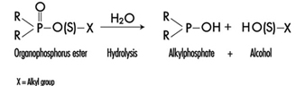
The determination in urine of metabolites that are derived from the alkyl phosphate moiety of the OP molecule or of the residues generated by the hydrolysis of the P–X bond (figure 1) has been used to monitor OP exposure.
Figure 1. Hydrolysis of OP insecticides
Alkyl phosphate metabolites.
The alkyl phosphate metabolites detectable in urine and the main parent compound from which they can originate are listed in table 5. Urinary alkyl phosphates are sensitive indicators of exposure to OP compounds: the excretion of these metabolites in urine is usually detectable at an exposure level at which plasma or erythrocyte cholinesterase inhibition cannot be detected. The urinary excretion of alkyl phosphates has been measured for different conditions of exposure and for various OP compounds (table 6). The existence of a relationship between external doses of OP and alkyl phosphate urinary concentrations has been established in a few studies. In some studies a significant relationship between cholinesterase activity and levels of alkyl phosphates in urine has also been demonstrated.
Table 5. Alkyl phosphates detectable in urine as metabolites of OP pesticides
|
Metabolite |
Abbreviation |
Principal parent compounds |
|
Monomethylphosphate |
MMP |
Malathion, parathion |
|
Dimethylphosphate |
DMP |
Dichlorvos, trichlorfon, mevinphos, malaoxon, dimethoate, fenchlorphos |
|
Diethylphosphate |
DEP |
Paraoxon, demeton-oxon, diazinon-oxon, dichlorfenthion |
|
Dimethylthiophosphate |
DMTP |
Fenitrothion, fenchlorphos, malathion, dimethoate |
|
Diethylthiophosphate |
DETP |
Diazinon, demethon, parathion,fenchlorphos |
|
Dimethyldithiophosphate |
DMDTP |
Malathion, dimethoate, azinphos-methyl |
|
Diethyldithiophosphate |
DEDTP |
Disulfoton, phorate |
|
Phenylphosphoric acid |
Leptophos, EPN |
Table 6. Examples of levels of urinary alkyl phosphates measured in various conditions of exposure to OP
|
Compound |
Condition of exposure |
Route of exposure |
Metabolite concentrations1 (mg/l) |
|
Parathion2 |
Nonfatal poisoning |
Oral |
DEP = 0.5 DETP = 3.9 |
|
Disulfoton2 |
Formulators |
Dermal/inhalation |
DEP = 0.01-4.40 DETP = 0.01-1.57 DEDTP = <0.01-.05 |
|
Phorate2 |
Formulators |
Dermal/inhalation |
DEP = 0.02-5.14 DETP = 0.08-4.08 DEDTP = <0.01-0.43 |
|
Malathion3 |
Sprayers |
Dermal |
DMDTP = <0.01 |
|
Fenitrothion3 |
Sprayers |
Dermal |
DMP = 0.01-0.42 DMTP = 0.02-0.49 |
|
Monocrotophos4 |
Sprayers |
Dermal/inhalation |
DMP = <0.04-6.3/24 h |
1 For abbreviations see table 27.12 [BMO12TE].
2 Dillon and Ho 1987.
3 Richter 1993.
4 van Sittert and Dumas 1990.
Alkyl phosphates are usually excreted in urine within a short time. Samples collected soon after the end of the workday are suitable for metabolite determination.
The measurement of alkyl phosphates in urine requires a rather sophisticated analytical method, based on derivatization of the compounds and detection by gas-liquid chromatography (Shafik et al. 1973a; Reid and Watts 1981).
Hydrolytic residues.
p-Nitrophenol (PNP) is the phenolic metabolite of parathion, methylparathion and ethyl parathion, EPN. The measurement of PNP in urine (Cranmer 1970) has been widely used and has proven to be successful in evaluating exposure to parathion. Urinary PNP correlates well with the absorbed dose of parathion. With PNP urinary levels up to 2 mg/l, the absorption of parathion does not cause symptoms, and little or no reduction of cholinesterase activities is observed. PNP excretion occurs rapidly and urinary levels of PNP become insignificant 48 hours after exposure. Thus, urine samples should be collected soon after exposure.
Carbamates
Biological indicators of effect.
Carbamate pesticides include insecticides, fungicides and herbicides. Insecticidal carbamate toxicity is due to the inhibition of synaptic ACHE, while other mechanisms of toxicity are involved for herbicidal and fungicidal carbamates. Thus, only exposure to carbamate insecticides can be monitored through the assay of cholinesterase activity in red blood cells (ACHE) or plasma (PCHE). ACHE is usually more sensitive to carbamate inhibitors than PCHE. Cholinergic symptoms have been usually observed in carbamate-exposed workers with a blood ACHE activity lower than 70% of the individual baseline level (WHO 1982a).
Inhibition of cholinesterases by carbamates is rapidly reversible. Therefore, false negative results can be obtained if too much time elapses between exposure and biological sampling or between sampling and analysis. In order to avoid such problems, it is recommended that blood samples be collected and analysed within four hours after exposure. Preference should be given to the analytical methods that allow the determination of cholinesterase activity immediately after blood sampling, as discussed for organophosphates.
Biological indicators of exposure.
The measurement of urinary excretion of carbamate metabolites as a method to monitor human exposure has so far been applied only to few compounds and in limited studies. Table 7 summarizes the relevant data. Since carbamates are promptly excreted in the urine, samples collected soon after the end of exposure are suitable for metabolite determination. Analytical methods for the measurements of carbamate metabolites in urine have been reported by Dawson et al. (1964); DeBernardinis and Wargin (1982) and Verberk et al. (1990).
Table 7. Levels of urinary carbamate metabolites measured in field studies
|
Compound |
Biological index |
Condition of exposure |
Environmental concentrations |
Results |
References |
|
Carbaryl |
a-naphthol a-naphthol a-naphthol |
formulators mixer/applicators unexposed population |
0.23–0.31 mg/m3 |
x=18.5 mg/l1 , max. excretion rate = 80 mg/day x=8.9 mg/l, range = 0.2–65 mg/l range = 1.5–4 mg/l |
WHO 1982a |
|
Pirimicarb |
metabolites I2 and V3 |
applicators |
range = 1–100 mg/l |
Verberk et al. 1990 |
1 Systemic poisonings have been occasionally reported.
2 2-dimethylamino-4-hydroxy-5,6-dimethylpyrimidine.
3 2-methylamino-4-hydroxy-5,6-dimethylpyrimidine.
x = standard deviation.
Dithiocarbamates
Biological indicators of exposure.
Dithiocarbamates (DTC) are widely used fungicides, chemically grouped in three classes: thiurams, dimethyldithiocarbamates and ethylene-bis-dithiocarbamates.
Carbon disulphide (CS2) and its main metabolite 2-thiothiazolidine-4-carboxylic acid (TTCA) are metabolites common to almost all DTC. A significant increase in urinary concentrations of these compounds has been observed for different conditions of exposure and for various DTC pesticides. Ethylene thiourea (ETU) is an important urinary metabolite of ethylene-bis-dithiocarbamates. It may also be present as an impurity in market formulations. Since ETU has been determined to be a teratogen and a carcinogen in rats and in other species and has been associated with thyroid toxicity, it has been widely applied to monitor ethylene-bis-dithiocarbamate exposure. ETU is not compound-specific, as it may be derived from maneb, mancozeb or zineb.
Measurement of the metals present in the DTC has been proposed as an alternative approach in monitoring DTC exposure. Increased urinary excretion of manganese has been observed in workers exposed to mancozeb (table 8).
Table 8. Levels of urinary dithiocarbamate metabolites measured in field studies
|
Compound |
Biological index |
Condition of exposure |
Environmental concentrations* ± standard deviation |
Results ± standard deviation |
References |
|
Ziram |
Carbon disulphide (CS2) TTCA1 |
formulators formulators |
1.03 ± 0.62 mg/m3 |
3.80 ± 3.70 mg/l 0.45 ± 0.37 mg/l |
Maroni et al. 1992 |
|
Maneb/Mancozeb |
ETU2 |
applicators |
range = < 0.2–11.8 mg/l |
Kurttio et al. 1990 |
|
|
Mancozeb |
Manganese |
applicators |
57.2 mg/m3 |
pre-exposure: 0.32 ± 0.23 mg/g creatinine; post-exposure: 0.53 ± 0.34 mg/g creatinine |
Canossa et al. 1993 |
* Mean result according to Maroni et al. 1992.
1 TTCA = 2-thiothiazolidine-4-carbonylic acid.
2 ETU = ethylene thiourea.
CS2, TTCA, and manganese are commonly found in urine of non-exposed subjects. Thus, the measurement of urinary levels of these compounds prior to exposure is recommended. Urine samples should be collected in the morning following the cessation of exposure. Analytical methods for the measurements of CS2, TTCA and ETU have been reported by Maroni et al. (1992).
Synthetic Pyrethroids
Biological indicators of exposure.
Synthetic pyrethroids are insecticides similar to natural pyrethrins. Urinary metabolites suitable for application in biological monitoring of exposure have been identified through studies with human volunteers. The acidic metabolite 3-(2,2’-dichloro-vinyl)-2,2’-dimethyl-cyclopropane carboxylic acid (Cl2CA) is excreted both by subjects orally dosed with permethrin and cypermethrin and the bromo-analogue (Br2CA) by subjects treated with deltamethrin. In the volunteers treated with cypermethrin, a phenoxy metabolite, 4-hydroxy-phenoxy benzoic acid (4-HPBA), has also been identified. These tests, however, have not often been applied in monitoring occupational exposures because of the complex analytical techniques required (Eadsforth, Bragt and van Sittert 1988; Kolmodin-Hedman, Swensson and Akerblom 1982). In applicators exposed to cypermethrin, urinary levels of Cl2CA have been found to range from 0.05 to 0.18 mg/l, while in formulators exposed to a-cypermethrin, urinary levels of 4-HPBA have been found to be lower than 0.02 mg/l.
A 24-hour urine collection period started after the end of exposure is recommended for metabolite determinations.
Organochlorines
Biological indicators of exposure.
Organochlorine (OC) insecticides were widely used in the 1950s and 1960s. Subsequently, the use of many of these compounds was discontinued in many countries because of their persistence and consequent contamination of the environment.
Biological monitoring of OC exposure can be carried out through the determination of intact pesticides or their metabolites in blood or serum (Dale, Curley and Cueto 1966; Barquet, Morgade and Pfaffenberger 1981). After absorption, aldrin is rapidly metabolized to dieldrin and can be measured as dieldrin in blood. Endrin has a very short half-life in blood. Therefore, endrin blood concentration is of use only in determining recent exposure levels. The determination of the urinary metabolite anti-12-hydroxy-endrin has also proven to be useful in monitoring endrin exposure (van Sittert and Tordoir 1987) .
Significant correlations between the concentration of biological indicators and the onset of toxic effects have been demonstrated for some OC compounds. Instances of toxicity due to aldrin and dieldrin exposure have been related to levels of dieldrin in blood above 200 μg/l. A blood lindane concentration of 20 μg/l has been indicated as the upper critical level as far as neurological signs and symptoms are concerned. No acute adverse effects have been reported in workers with blood endrin concentrations below 50 μg/l. Absence of early adverse effects (induction of liver microsomal enzymes) has been shown on repeated exposures to endrin at urinary anti-12-hydroxy-endrin concentrations below 130 μg/g creatinine and on repeated exposures to DDT at DDT or DDE serum concentrations below 250 μg/l.
OC may be found in low concentrations in the blood or urine of the general population. Examples of observed values are as follows: lindane blood concentrations up to 1 μg/l, dieldrin up to 10 μg/l, DDT or DDE up to 100 μg/l, and anti-12-hydroxy-endrin up to 1 μg/g creatinine. Thus, a baseline assessment prior to exposure is recommended.
For exposed subjects, blood samples should be taken immediately after the end of a single exposure. For conditions of long-term exposure, the time of collection of the blood sample is not critical. Urine spot samples for urinary metabolite determination should be collected at the end of exposure.
Triazines
Biological indicators of exposure.
The measurement of urinary excretion of triazinic metabolites and the unmodified parent compound has been applied to subjects exposed to atrazine in limited studies. Figure 2 shows the urinary excretion profiles of atrazine metabolites of a manufacturing worker with dermal exposure to atrazine ranging from 174 to 275 μmol/workshift (Catenacci et al. 1993). Since other chlorotriazines (simazine, propazine, terbuthylazine) follow the same biotransformation pathway of atrazine, levels of dealkylated triazinic metabolites may be determined to monitor exposure to all chlorotriazine herbicides.
Figure 2. Urinary excretion profiles of atrazine metabolites

The determination of unmodified compounds in urine may be useful as a qualitative confirmation of the nature of the compound that has generated the exposure. A 24–hour urine collection period started at the beginning of exposure is recommended for metabolite determination.
Recently, by using an enzyme-linked immunosorbent assay (ELISA test), a mercapturic acid conjugate of atrazine has been identified as its major urinary metabolite in exposed workers. This compound has been found in concentrations at least 10 times higher than those of any dealkylated products. A relationship between cumulative dermal and inhalation exposure and total amount of the mercapturic acid conjugate excreted over a 10-day period has been observed (Lucas et al. 1993).
Coumarin Derivatives
Biological indicators of effect.
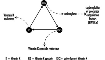
Coumarin rodenticides inhibit the activity of the enzymes of the vitamin K cycle in the liver of mammals, humans included (figure 3), thus causing a dose-related reduction of the synthesis of vitamin K-dependent clotting factors, namely factor II (prothrombin), VII, IX, and X. Anticoagulant effects appear when plasma levels of clotting factors have dropped below approximately 20% of normal.
Figure 3. Vitamin K cycle
These vitamin K antagonists have been grouped into so-called “first generation” (e.g., warfarin) and “second generation” compounds (e.g., brodifacoum, difenacoum), the latter characterized by a very long biological half-life (100 to 200 days).
The determination of prothrombin time is widely used in monitoring exposure to coumarins. However, this test is sensitive only to a clotting factor decrease of approximately 20% of normal plasma levels. The test is not suitable for detection of early effects of exposure. For this purpose, the determination of the prothrombin concentration in plasma is recommended.
In the future, these tests might be replaced by the determination of coagulation factor precursors (PIVKA), which are substances detectable in blood only in the case of blockage of the vitamin K cycle by coumarins.
With conditions of prolonged exposure, the time of blood collection is not critical. In cases of acute overexposure, biological monitoring should be carried out for at least five days after the event, in view of the latency of the anticoagulant effect. To increase the sensitivity of these tests, the measurement of baseline values prior to exposure is recommended.
Biological indicators of exposure.
The measurement of unmodified coumarins in blood has been proposed as a test to monitor human exposure. However, experience in applying these indices is very limited mainly because the analytical techniques are much more complex (and less standardized) in comparison with those required to monitor the effects on the coagulation system (Chalermchaikit, Felice and Murphy 1993).
Phenoxy Herbicides
Biological indicators of exposure.
Phenoxy herbicides are scarcely biotransformed in mammals. In humans, more than 95% of a 2,4-dichlorophenoxyacetic acid (2,4-D) dose is excreted unchanged in urine within five days, and 2,4,5-trichlorophenoxyacetic acid (2,4,5-T) and 4-chloro-2-methylphenoxyacetic acid (MCPA) are also excreted mostly unchanged via urine within a few days after oral absorption. The measurement of unchanged compounds in urine has been applied in monitoring occupational exposure to these herbicides. In field studies, urinary levels of exposed workers have been found to range from 0.10 to 8 μg/l for 2,4-D, from 0.05 to 4.5 μg/l for 2,4,5-T and from below 0.1 μg/l to 15 μg/l for MCPA. A 24-hour period of urine collection starting at the end of exposure is recommended for the determination of unchanged compounds. Analytical methods for the measurements of phenoxy herbicides in urine have been reported by Draper (1982).
Quaternary Ammonium Compounds
Biological indicators of exposure.
Diquat and paraquat are herbicides scarcely biotransformed by the human organism. Because of their high water solubility, they are readily excreted unchanged in urine. Urine concentrations below the analytical detection limit (0.01 μg/l) have been often observed in paraquat exposed workers; while in tropical countries, concentrations up to 0.73 μg/l have been measured after improper paraquat handling. Urinary diquat concentrations lower than the analytical detection limit (0.047 μg/l) have been reported for subjects with dermal exposures from 0.17 to 1.82 μg/h and inhalation exposures lower than 0.01 μg/h. Ideally, 24 hours sampling of urine collected at the end of exposure should be used for analysis. When this is impractical, a spot sample at the end of the workday can be used.
Determination of paraquat levels in serum is useful for prognostic purposes in case of acute poisoning: patients with serum paraquat levels up to 0.1 μg/l twenty-four hours after ingestion are likely to survive.
The analytical methods for paraquat and diquat determination have been reviewed by Summers (1980).
Miscellaneous Pesticides
4,6-Dinitro-o-cresol (DNOC).
DNOC is an herbicide introduced in 1925, but the use of this compound has been progressively decreased due to its high toxicity to plants and to humans. Since blood DNOC concentrations correlate to a certain extent with the severity of adverse health effects, the measure of unchanged DNOC in blood has been proposed for monitoring occupational exposures and for the evaluation of the clinical course of poisonings.
Pentachlorophenol.
Pentachlorophenol (PCP) is a wide-spectrum biocide with pesticidal action against weeds, insects, and fungi. Measurements of blood or urinary unchanged PCP have been recommended as suitable indices in monitoring occupational exposures (Colosio et al. 1993), because these parameters are significantly correlated with PCP body burden. In workers with prolonged exposure to PCP the time of blood collection is not critical, while urine spot samples should be collected on the morning after exposure.
A multiresidue method for the measurement of halogenated and nitrophenolic pesticides has been described by Shafik et al.(1973b).
Other tests proposed for the biological monitoring of pesticide exposure are listed in table 9.
Table 9. Other indices proposed in the literature for the biological monitoring of pesticide exposure
|
Compound |
Biological index |
|
|
Urine |
Blood |
|
|
Bromophos |
Bromophos |
Bromophos |
|
Captan |
Tetrahydrophtalimide |
|
|
Carbofuran |
3-Hydroxycarbofuran |
|
|
Chlordimeform |
4-Chloro-o-toluidine derivatives |
|
|
Chlorobenzilate |
p,p-1-Dichlorobenzophenone |
|
|
Dichloropropene |
Mercapturic acid metabolites |
|
|
Fenitrothion |
p-Nitrocresol |
|
|
Ferbam |
Thiram |
|
|
Fluazifop-Butyl |
Fluazifop |
|
|
Flufenoxuron |
Flufenoxuron |
|
|
Glyphosate |
Glyphosate |
|
|
Malathion |
Malathion |
Malathion |
|
Organotin compounds |
Tin |
Tin |
|
Trifenomorph |
Morpholine, triphenylcarbinol |
|
|
Ziram |
Thiram |
|
Conclusions
Biological indicators for monitoring pesticide exposure have been applied in a number of experimental and field studies.
Some tests, such as those for cholinesterase in blood or for selected unmodified pesticides in urine or blood, have been validated by extensive experience. Biological exposure limits have been proposed for these tests (table 10). Other tests, in particular those for blood or urinary metabolites, suffer from greater limitations because of analytical difficulties or because of limitations in interpretation of results.
Table 10. Recommended biological limit values (as of 1996)
|
Compound |
Biological index |
BEI1 |
BAT2 |
HBBL3 |
BLV4 |
|
ACHE inhibitors |
ACHE in blood |
70% |
70% |
70%, |
|
|
DNOC |
DNOC in blood |
20 mg/l, |
|||
|
Lindane |
Lindane in blood |
0.02mg/l |
0.02mg/l |
||
|
Parathion |
PNP in urine |
0.5mg/l |
0.5mg/l |
||
|
Pentachlorophenol (PCP) |
PCP in urine PCP in plasma |
2 mg/l 5 mg/l |
0.3mg/l 1 mg/l |
||
|
Dieldrin/Aldrin |
Dieldrin in blood |
100 mg/l |
|||
|
Endrin |
Anti-12-hydroxy-endrin in urine |
130 mg/l |
|||
|
DDT |
DDT and DDEin serum |
250 mg/l |
|||
|
Coumarins |
Prothrombin time in plasma Prothrombin concentration in plasma |
10% above baseline 60% of baseline |
|||
|
MCPA |
MCPA in urine |
0.5 mg/l |
|||
|
2,4-D |
2,4-D in urine |
0.5 mg/l |
1 Biological exposure indices (BEIs) are recommended by the American Conference of Governmental Industrial Hygienists (ACGIH 1995).
2 Biological tolerance values (BATs) are recommended by the German Commission for the Investigation of Health Hazards of Chemical Compounds in the Work Area (DFG 1992).
3 Health-based biological limits (HBBLs) are recommended by a WHO Study Group (WHO 1982a).
4 Biological limit values (BLVs) are proposed by a Study Group of the Scientific Committee on Pesticides of the International Commission on Occupational Health (Tordoir et al. 1994). Assessment of working conditions is called for if this value is exceeded.
This field is in rapid development and, given the enormous importance of using biological indicators to assess exposure to these substances, new tests will be continuously developed and validated.
Epidemiological Method Applied to Occupational Health and Safety
Epidemiology
Epidemiology is recognized both as the science basic to preventive medicine and one that informs the public health policy process. Several operational definitions of epidemiology have been suggested. The simplest is that epidemiology is the study of the occurrence of disease or other health-related characteristics in human and in animal populations. Epidemiologists study not only the frequency of disease, but whether the frequency differs across groups of people; i.e., they study the cause-effect relationship between exposure and illness. Diseases do not occur at random; they have causes—quite often man-made causes—which are avoidable. Thus, many diseases could be prevented if the causes were known. The methods of epidemiology have been crucial to identifying many causative factors which, in turn, have led to health policies designed to prevent disease, injury and premature death.
What is the task of epidemiology and what are its strengths and weaknesses when definitions and concepts of epidemiology are applied to occupational health? This chapter addresses these questions and the ways in which occupational health hazards can be investigated using epidemiological techniques. This article introduces the ideas found in successive articles in this chapter.
Occupational Epidemiology
Occupational epidemiology has been defined as the study of the effects of workplace exposures on the frequency and distribution of diseases and injuries in the population. Thus it is an exposure-oriented discipline with links to both epidemiology and occupational health (Checkoway et al. 1989). As such, it uses methods similar to those employed by epidemiology in general.
The main objective of occupational epidemiology is prevention through identifying the consequences of workplace exposures on health. This underscores the preventive focus of occupational epidemiology. Indeed, all research in the field of occupational health and safety should serve preventive purposes. Hence, epidemiological knowledge can and should be readily implementable. While the public health interest always should be the primary concern of epidemiological research, vested interests can exercise influence, and care must be taken to minimize such influence in the formulation, conduct and/or interpretation of studies (Soskolne 1985; Soskolne 1989).
A second objective of occupational epidemiology is to use results from specific settings to reduce or to eliminate hazards in the population at large. Thus, apart from providing information on the health effects of exposures in the workplace, the results from occupational epidemiology studies also play a role in the estimation of risk associated with the same exposures but at the lower levels generally experienced by the general population. Environmental contamination from industrial processes and products usually would result in lower levels of exposure than those experienced in the workplace.
The levels of application of occupational epidemiology are:
- surveillance to describe the occurrence of illness in different categories of workers and so provide early warning signals of unrecognized occupational hazards
- generation and testing of an hypothesis that a given exposure may be harmful, and the quantification of an effect
- evaluation of an intervention (for example, a preventive action such as reduction in exposure levels) by measuring changes in the health status of a population over time.
The causal role that occupational exposures can play in the development of disease, injury and premature death had been identified long ago and is part of the history of epidemiology. Reference has to be made to Bernardino Ramazzini, founder of occupational medicine and one of the first to revive and add to the Hippocratic tradition of the dependence of health on identifiable natural external factors. In the year 1700, he wrote in his “De Morbis Artificum Diatriba” (Ramazzini 1705; Saracci 1995):
The physician has to ask many questions of the patients. Hippocrates states in De Affectionibus: “When you face a sick person you should ask him from what he is suffering, for what reason, for how many days, what he eats, and what are his bowel movements. To all these questions one should be added: ‘What work does he do?’.”
This reawakening of clinical observation and of the attention to the circumstances surrounding the occurrence of disease, brought Ramazzini to identify and describe many of the occupational diseases that were later studied by occupational physicians and epidemiologists.
Using this approach, Pott was first to report in 1775 (Pott 1775) the possible connection between cancer and occupation (Clayson 1962). His observations on cancer of the scrotum among chimney-sweeps began with a description of the disease and continued:
The fate of these people seems singularly hard: in their early infancy, they are most frequently treated with great brutality, and almost starved with cold and hunger; they are thrust up narrow, and sometimes hot chimneys, where they are bruised, burned and almost suffocated; and when they get to puberty, become peculiarly liable to a most noisome, painful, and fatal disease.
Of this last circumstance there is not the least doubt, though perhaps it may not have been sufficiently attended to, to make it generally known. Other people have cancer of the same parts; and so have others, besides lead-workers, the Poitou colic, and the consequent paralysis; but it is nevertheless a disease to which they are peculiarly liable; and so are chimney-sweeps to cancer of the scrotum and testicles.
The disease, in these people, seems to derive its origin from a lodgement of soot in the rugae of the scrotum, and at first not to be a disease of the habit … but here the subjects are young, in general good health, at least at first; the disease brought on them by their occupation, and in all probability local; which last circumstance may, I think, be fairly presumed from its always seizing the same parts; all this makes it (at first) a very different case from a cancer which appears in an elderly man.
This first account of an occupational cancer still remains a model of lucidity. The nature of the disease, the occupation concerned and the probable causal agent are all clearly defined. An increased incidence of scrotal cancer among chimney-sweeps is noted although no quantitative data are given to substantiate the claim.
Another fifty years passed before Ayrton-Paris noticed in 1822 (Ayrton-Paris 1822) the frequent development of scrotal cancers among the copper and tin smelters of Cornwall, and surmised that arsenic fumes might be the causal agent. Von Volkmann reported in 1874 skin tumours in paraffin workers in Saxony, and shortly afterwards, Bell suggested in 1876 that shale oil was responsible for cutaneous cancer (Von Volkmann 1874; Bell 1876). Reports of the occupational origin of cancer then became relatively more frequent (Clayson 1962).
Among the early observations of occupational diseases was the increased occurrence of lung cancer among Schneeberg miners (Harting and Hesse 1879). It is noteworthy (and tragic) that a recent case study shows that the epidemic of lung cancer in Schneeberg is still a huge public health problem, more than a century after the first observation in 1879. An approach to identify an “increase” in disease and even to quantify it had been present in the history of occupational medicine. For example, as Axelson (1994) has pointed out, W.A. Guy in 1843 studied “pulmonary consumption” in letter press printers and found a higher risk among compositors than among pressmen; this was done by applying a design similar to the case-control approach (Lilienfeld and Lilienfeld 1979). Nevertheless, it was not until perhaps the early 1950s that modern occupational epidemiology and its methodology began to develop. Major contributions marking this development were the studies on bladder cancer in dye workers (Case and Hosker 1954) and lung cancer among gas workers (Doll 1952).
Issues in Occupational Epidemiology
The articles in this chapter introduce both the philosophy and the tools of epidemiological investigation. They focus on assessing the exposure experience of workers and on the diseases that arise in these populations. Issues in drawing valid conclusions about possible causative links in the pathway from exposures to hazardous substances to the development of diseases are addressed in this chapter.
Ascertainment of an individual’s work life exposure experience constitutes the core of occupational epidemiology. The informativeness of an epidemiological study depends, in the first instance, on the quality and extent of available exposure data. Secondly, the health effects (or, the diseases) of concern to the occupational epidemiologist must be accurately determinable among a well-defined and accessible group of workers. Finally, data about other potential influences on the disease of interest should be available to the epidemiologist so that any occupational exposure effects that are established from the study can be attributed to the occupational exposure per se rather than to other known causes of the disease in question. For example, in a group of workers who may work with a chemical that is suspected of causing lung cancer, some workers may also have a history of tobacco smoking, a further cause of lung cancer. In the latter situation, occupational epidemiologists must determine which exposure (or, which risk factor—the chemical or the tobacco, or, indeed, the two in combination) is responsible for any increase in the risk of lung cancer in the group of workers being studied.
Exposure assessment
If a study has access only to the fact that a worker was employed in a particular industry, then the results from such a study can link health effects only to that industry. Likewise, if knowledge about exposure exists for the occupations of the workers, conclusions can be directly drawn only in so far as occupations are concerned. Indirect inferences on chemical exposures can be made, but their reliability has to be evaluated situation by situation. If a study has access, however, to information about the department and/or job title of each worker, then conclusions will be able to be made to that finer level of workplace experience. Where information about the actual substances with which a person works is known to the epidemiologist (in collaboration with an industrial hygienist), then this would be the finest level of exposure information available in the absence of rarely available dosimetry. Furthermore, the findings from such studies can provide more useful information to industry for creating safer workplaces.
Epidemiology has been a sort of “black box” discipline until now, because it has studied the relationship between exposure and disease (the two extremes of the causal chain), without considering the intermediate mechanistic steps. This approach, despite its apparent lack of refinement, has been extremely useful: in fact, all the known causes of cancer in humans, for instance, have been discovered with the tools of epidemiology.
The epidemiological method is based on available records —questionnaires, job titles or other “proxies” of exposure; this makes the conduct of epidemiological studies and the interpretation of their findings relatively simple.
Limitations of the more crude approach to exposure assessment, however, have become evident in recent years, with epidemiologists facing more complex problems. Limiting our consideration to occupational cancer epidemiology, most well-known risk factors have been discovered because of high levels of exposure in the past; a limited number of exposures for each job; large populations of exposed workers; and a clear-cut correspondence between “proxy” information and chemical exposures (e.g., shoe workers and benzene, shipyards and asbestos, and so on). Nowadays, the situation is substantially different: levels of exposure are considerably lower in Western countries (this qualification should always be stressed); workers are exposed to many different chemicals and mixtures in the same job title (e.g., agricultural workers); homogeneous populations of exposed workers are more difficult to find and are usually small in number; and, the correspondence between “proxy” information and actual exposure grows progressively weaker. In this context, the tools of epidemiology have reduced sensitivity owing to the misclassification of exposure.
In addition, epidemiology has relied on “hard” end points, such as death in most cohort studies. However, workers might prefer to see something different from “body counts” when the potential health effects of occupational exposures are studied. Therefore, the use of more direct indicators of both exposure and early response would have some advantages. Biological markers may provide just a tool.
Biological markers
The use of biological markers, such as lead levels in blood or liver function tests, is not new in occupational epidemiology. However, the utilization of molecular techniques in epidemiological studies has made possible the use of biomarkers for assessing target organ exposures, for determining susceptibility and for establishing early disease.
Potential uses of biomarkers in the context of occupational epidemiology are:
- exposure assessment in cases in which traditional epidemiological tools are insufficient (particularly for low doses and low risks)
- to disentangle the causative role of single chemical agents or substances in multiple exposures or mixtures
- estimation of the total burden of exposure to chemicals having the same mechanistic target
- investigation of pathogenetic mechanisms
- study of individual susceptibility (e.g., metabolic polymorphisms, DNA repair) (Vineis 1992)
- to classify exposure and/or disease more accurately, thereby increasing statistical power.
Great enthusiasm has arisen in the scientific community about these uses, but, as noted above, methodological complexity of the use of these new “molecular tools” should serve to caution against excessive optimism. Biomarkers of chemical exposures (such as DNA adducts) have several shortcomings:
- They usually reflect recent exposures and, therefore, are of limited use in case-control studies, whereas they require repeated samplings over prolonged periods for utilization in cohort investigations.
- While they can be highly specific and thus improve exposure misclassification, findings often remain difficult to interpret.
- When complex chemical exposures are investigated (e.g., air pollution or environmental tobacco smoke) it is possible that the biomarker would reflect one particular component of the mixture, whereas the biological effect could be due to another.
- In many situations, it is not clear whether a biomarker reflects a relevant exposure, a correlate of the relevant exposure, individual susceptibility, or an early disease stage, thus limiting causal inference.
- The determination of most biomarkers requires an expensive test or an invasive procedure or both, thus creating constraints for adequate study size and statistical power.
- A biomarker of exposure is no more than a proxy for the real objective of an epidemiological investigation, which, as a rule, focuses on an avoidable environmental exposure (Trichopoulos 1995; Pearce et al. 1995).
Even more important than the methodological shortcomings is the consideration that molecular techniques might cause us to redirect our focus from identifying risks in the exogenous environment, to identifying high-risk individuals and then making personalized risk assessments by measuring phenotype, adduct load and acquired mutations. This would direct our focus, as noted by McMichael, to a form of clinical evaluation, rather than one of public health epidemiology. Focusing on individuals could distract us from the important public health goal of creating a less hazardous environment (McMichael 1994).
Two further important issues emerge regarding the use of biomarkers:
- The use of biomarkers in occupational epidemiology must be accompanied by a clear policy as far as informed consent is concerned. The worker may have several reasons to refuse cooperation. One very practical reason is that the identification of, say, an alteration in an early response marker such as sister chromatid exchange implies the possibility of discrimination by health and life insurers and by employers who might shun the worker because he or she may be more prone to disease. A second reason concerns genetic screening: since the distributions of genotypes and phenotypes vary according to ethnic group, occupational opportunities for minorities might be hampered by genetic screening. Third, doubts can be raised about the predictability of genetic tests: since the predictive value depends on the prevalence of the condition which the test aims to identify, if the latter is rare, the predictive value will be low and the practical use of the screening test will be questionable. Until now, none of the genetic screening tests have been judged applicable in the field (Ashford et al. 1990).
- Ethical principles must be applied prior to the use of biomarkers. These principles have been evaluated for biomarkers used for identifying individual susceptibility to disease by an interdisciplinary Working Group of the Technical Office of the European Trade Unions, with the support of the Commission of the European Communities (Van Damme et al. 1995); their report has reinforced the view that tests can be conducted only with the objective of preventing disease in a workforce. Among other considerations, use of tests must never.
- serve as a means for “selection of the fittest”
- be used to avoid implementing effective preventive measures, such as the identification and substitution of risk factors or improvements in conditions in the workplace
- create, confirm or reinforce social inequality
- create a gap between the ethical principles followed in the workplace and the ethical principles that must be upheld in a democratic society
- oblige a person seeking employment to disclose personal details other than those strictly necessary for obtaining the job.
Finally, evidence is accumulating that the metabolic activation or inactivation of hazardous substances (and of carcinogens in particular) varies considerably in human populations, and is partly genetically determined. Furthermore, inter-individual variability in the susceptibility to carcinogens may be particularly important at low levels of occupational and environmental exposure (Vineis et al. 1994). Such findings may strongly affect regulatory decisions that focus the risk assessment process on the most susceptible (Vineis and Martone 1995).
Study design and validity
Hernberg’s article on epidemiological study designs and their applications in occupational medicine concentrates on the concept of “study base”, defined as the morbidity experience (in relation to some exposure) of a population while it is followed over time. Thus, the study base is not only a population (i.e., a group of people), but the experience of disease occurrence of this population during a certain period of time (Miettinen 1985, Hernberg 1992). If this unifying concept of a study base is adopted, then it is important to recognize that the different study designs (e.g., case-control and cohort designs) are simply different ways of “harvesting” information on both exposure and disease from the same study base; they are not diametrically different approaches.
The article on validity in study design by Sasco addresses definitions and the importance of confounding. Study investigators must always consider the possibility of confounding in occupational studies, and it can never be sufficiently stressed that the identification of potentially confounding variables is an integral part of any study design and analysis. Two aspects of confounding must be addressed in occupational epidemiology:
- Negative confounding should be explored: for example, some industrial populations have low exposure to lifestyle-associated risk factors because of a smoke-free workplace; glass blowers tend to smoke less than the general population.
- When confounding is considered, an estimate of its direction and its potential impact ought to be assessed. This is particularly true when data to control confounding are scanty. For example, smoking is an important confounder in occupational epidemiology and it always should be considered. Nevertheless, when data on smoking are not available (as is often the case in cohort studies), it is unlikely that smoking can explain a large excess of risk found in an occupational group. This is nicely described in a paper by Axelson (1978) and further discussed by Greenland (1987). When detailed data on both occupation and smoking have been available in the literature, confounding did not seem to heavily distort the estimates concerning the association between lung cancer and occupation (Vineis and Simonato 1991). Furthermore, suspected confounding does not always introduce non-valid associations. Since investigators also are at risk of being led astray by other undetected observation and selection biases, these should receive as much emphasis as the issue of confounding in designing a study (Stellman 1987).
Time and time-related variables such as age at risk, calendar period, time since hire, time since first exposure, duration of exposure and their treatment at the analysis stage, are among the most complex methodological issues in occupational epidemiology. They are not covered in this chapter, but two relevant and recent methodological references are noted (Pearce 1992; Robins et al. 1992).
Statistics
The article on statistics by Biggeri and Braga, as well as the title of this chapter, indicate that statistical methods cannot be separated from epidemiological research. This is because: (a) a sound understanding of statistics may provide valuable insights into the proper design of an investigation and (b) statistics and epidemiology share a common heritage, and the entire quantitative basis of epidemiology is grounded in the notion of probability (Clayton 1992; Clayton and Hills 1993). In many of the articles that follow, empirical evidence and proof of hypothesized causal relationships are evaluated using probabilistic arguments and appropriate study designs. For example, emphasis is placed on estimating the risk measure of interest, like rates or relative risks, and on the construction of confidence intervals around these estimates instead of the execution of statistical tests of probability (Poole 1987; Gardner and Altman 1989; Greenland 1990). A brief introduction to statistical reasoning using the binomial distribution is provided. Statistics should be a companion to scientific reasoning. But it is worthless in the absence of properly designed and conducted research. Statisticians and epidemiologists are aware that the choice of methods determines what and the extent to which we make observations. The thoughtful choice of design options is therefore of fundamental importance in order to ensure valid observations.
Ethics
The last article, by Vineis, addresses ethical issues in epidemiological research. Points to be mentioned in this introduction refer to epidemiology as a discipline that implies preventive action by definition. Specific ethical aspects with regard to the protection of workers and of the population at large require recognition that:
- Epidemiological studies in occupational settings should in no way delay preventive measures in the workplace.
- Occupational epidemiology does not refer to lifestyle factors, but to situations where usually little or no personal role is played in the choice of exposure. This implies a particular commitment to effective prevention and to the immediate transmission of information to workers and the public.
- Research uncovers health hazards and provides the knowledge for preventive action. The ethical problems of not carrying out research, when it is feasible, should be considered.
- Notification to workers of the results of epidemiological studies is both an ethical and methodological issue in risk communication. Research in evaluating the potential impact and effectiveness of notification should be given high priority (Schulte et al. 1993).
Training in occupational epidemiology
People with a diverse range of backgrounds can find their way into the specialization of occupational epidemiology. Medicine, nursing and statistics are some of the more likely backgrounds seen among those specializing in this area. In North America, about half of all trained epidemiologists have science backgrounds, while the other half will have proceeded along the doctor of medicine path. In countries outside North America, most specialists in occupational epidemiology will have advanced through the doctor of medicine ranks. In North America, those with medical training tend to be considered “content experts”, while those who are trained through the science route are deemed “methodological experts”. It is often advantageous for a content expert to team up with a methodological expert in order to design and conduct the best possible study.
Not only is knowledge of epidemiological methods, statistics and computers needed for the occupational epidemiology speciality, but so is knowledge of toxicology, industrial hygiene and disease registries (Merletti and Comba 1992). Because large studies can require linkage to disease registries, knowledge of sources of population data is useful. Knowledge of labour and corporate organization also is important. Theses at the masters level and dissertations at the doctoral level of training equip students with the knowledge needed for conducting large record-based and interview-based studies among workers.
Proportion of disease attributable to occupation
The proportion of disease which is attributable to occupational exposures either in a group of exposed workers or in the general population is covered at least with respect to cancer in another part of this Encyclopaedia. Here we should remember that if an estimate is computed, it should be for a specific disease (and a specific site in the case of cancer), a specific time period and a specific geographic area. Furthermore, it should be based on accurate measures of the proportion of exposed people and the degree of exposure. This implies that the proportion of disease attributable to occupation may vary from very low or zero in certain populations to very high in others located in industrial areas where, for example, as much as 40% of lung cancer can be attributable to occupational exposures (Vineis and Simonato 1991). Estimates which are not based on a detailed review of well-designed epidemiological studies can, at the very best, be considered as informed guesses, and are of limited value.
Transfer of hazardous industries
Most epidemiological research is carried out in the developed world, where regulation and control of known occupational hazards has reduced the risk of disease over the past several decades. At the same time, however, there has been a large transfer of hazardous industries to the developing world (Jeyaratnam 1994). Chemicals previously banned in the United States or Europe now are produced in developing countries. For example, asbestos milling has been transferred from the US to Mexico, and benzidine production from European countries to the former Yugoslavia and Korea (Simonato 1986; LaDou 1991; Pearce et al. 1994).
An indirect sign of the level of occupational risk and of the working conditions in the developing world is the epidemic of acute poisoning taking place in some of these countries. According to one assessment, there are about 20,000 deaths each year in the world from acute pesticide intoxication, but this is likely to be a substantial underestimate (Kogevinas et al. 1994). It has been estimated that 99% of all deaths from acute pesticide poisoning occur in developing countries, where only 20% of the world’s agrochemicals are used (Kogevinas et al. 1994). This is to say that even if the epidemiological research seems to point to a reduction of occupational hazards, this might simply be due to the fact that most of this research is being conducted in the developed world. The occupational hazards may simply have been transferred to the developing world and the total world occupational exposure burden might have increased (Vineis et al. 1995).
Veterinary epidemiology
For obvious reasons, veterinary epidemiology is not directly pertinent to occupational health and occupational epidemiology. Nevertheless, clues to environmental and occupational causes of diseases may come from epidemiological studies on animals for several reasons:
- The life span of animals is relatively short compared with that of humans, and the latency period for diseases (e.g., most cancers) is shorter in animals than in humans. This implies that a disease that occurs in a wild or pet animal can serve as a sentinel event to alert us to the presence of a potential environmental toxicant or carcinogen for humans before it would have been identified by other means (Glickman 1993).
- Markers of exposures, such as haemoglobin adducts or levels of absorption and excretion of toxins, may be measured in wild and pet animals to assess environmental contamination from industrial sources (Blondin and Viau 1992; Reynolds et al. 1994; Hungerford et al. 1995).
- Animals are not exposed to some factors which may act as confounders in human studies, and investigations in animal populations therefore can be conducted without regard to these potential confounders. For example, a study of lung cancer in pet dogs might detect significant associations between the disease and exposure to asbestos (e.g., via owners’ asbestos-related occupations and proximity to industrial sources of asbestos). Clearly, such a study would remove the effect of active smoking as a confounder.
Veterinarians talk about an epidemiological revolution in veterinary medicine (Schwabe 1993) and textbooks about the discipline have appeared (Thrusfield 1986; Martin et al. 1987). Certainly, clues to environmental and occupational hazards have come from the joint efforts of human and animal epidemiologists. Among others, the effect of phenoxyherbicides in sheep and dogs (Newell et al. 1984; Hayes et al. 1990), of magnetic fields (Reif et al. 1995) and pesticides (notably flea preparations) contaminated with asbestos-like compounds in dogs (Glickman et al. 1983) are notable contributions.
Participatory research, communicating results and prevention
It is important to recognize that many epidemiological studies in the field of occupational health are initiated through the experience and concern of workers themselves (Olsen et al. 1991). Often, the workers—those historically and/or presently exposed—believed that something was wrong long before this was confirmed by research. Occupational epidemiology can be thought of as a way of “making sense” of the workers’ experience, of collecting and grouping the data in a systematic way, and allowing inferences to be made about the occupational causes of their ill health. Furthermore, the workers themselves, their representatives and the people in charge of workers’ health are the most appropriate persons to interpret the data which are collected. They therefore should always be active participants in any investigation conducted in the workplace. Only their direct involvement will guarantee that the workplace will remain safe after the researchers have left. The aim of any study is the use of the results in the prevention of disease and disability, and the success of this depends to a large extent on ensuring that the exposed participate in obtaining and interpreting the results of the study. The role and use of research findings in the litigation process as workers seek compensation for damages caused through workplace exposure is beyond the scope of this chapter. For some insight on this, the reader is referred elsewhere (Soskolne, Lilienfeld and Black 1994).
Participatory approaches to ensuring the conduct of occupational epidemiological research have in some places become standard practice in the form of steering committees established to oversee the research initiative from its inception to its completion. These committees are multipartite in their structure, including labour, science, management and/or government. With representatives of all stakeholder groups in the research process, the communication of results will be made more effective by virtue of their enhanced credibility because “one of their own” would have been overseeing the research and would be communicating the findings to his or her respective constituency. In this way, the greatest level of effective prevention is likely.
These and other participatory approaches in occupational health research are undertaken with the involvement of those who experience or are otherwise affected by the exposure-related problem of concern. This should be seen more commonly in all epidemiological research (Laurell et al. 1992). It is relevant to remember that while in epidemiological work the objective of analysis is estimation of the magnitude and distribution of risk, in participatory research, the preventability of the risk is also an objective (Loewenson and Biocca 1995). This complementarity of epidemiology and effective prevention is part of the message of this Encyclopaedia and of this chapter.
Maintaining public health relevance
Although new developments in epidemiological methodology, in data analysis and in exposure assessment and measurement (such as new molecular biological techniques) are welcome and important, they can also contribute to a reductionist approach focusing on individuals, rather than on populations. It has been said that:
… epidemiology has largely ceased to function as part of a multidisciplinary approach to understanding the causation of disease in populations and has become a set of generic methods for measuring associations of exposure and disease in individuals.… There is current neglect of social, economic, cultural, historical, political and other population factors as major causes of diseases.…Epidemiology must reintegrate itself into public health, and must rediscover the population perspective (Pearce 1996).
Occupational and environmental epidemiologists have an important role to play, not only in developing new epidemiological methods and applications for these methods, but also in ensuring that these methods are always integrated in the proper population perspective.
Anthropometry
This article is adapted from the 3rd edition of the Encyclopaedia of Occupational Health and Safety.
Anthropometry is a fundamental branch of physical anthropology. It represents the quantitative aspect. A wide system of theories and practice is devoted to defining methods and variables to relate the aims in the different fields of application. In the fields of occupational health, safety and ergonomics anthropometric systems are mainly concerned with body build, composition and constitution, and with the dimensions of the human body’s interrelation to workplace dimensions, machines, the industrial environment, and clothing.
Anthropometric variables
An anthropometric variable is a measurable characteristic of the body that can be defined, standardized and referred to a unit of measurement. Linear variables are generally defined by landmarks that can be precisely traced to the body. Landmarks are generally of two types: skeletal-anatomical, which may be found and traced by feeling bony prominences through the skin, and virtual landmarks that are simply found as maximum or minimum distances using the branches of a caliper.
Anthropometric variables have both genetic and environmental components and may be used to define individual and population variability. The choice of variables must be related to the specific research purpose and standardized with other research in the same field, as the number of variables described in the literature is extremely large, up to 2,200 having been described for the human body.
Anthropometric variables are mainly linear measures, such as heights, distances from landmarks with subject standing or seated in standardized posture; diameters, such as distances between bilateral landmarks; lengths, such as distances between two different landmarks; curved measures, namely arcs, such as distances on the body surface between two landmarks; and girths, such as closed all-around measures on body surfaces, generally positioned at at least one landmark or at a defined height.
Other variables may require special methods and instruments. For instance skinfold thickness is measured by means of special constant pressure calipers. Volumes are measured by calculation or by immersion in water. To obtain full information on body surface characteristics, a computer matrix of surface points may be plotted using biostereometric techniques.
Instruments
Although sophisticated anthropometric instruments have been described and used with a view to automated data collection, basic anthropometric instruments are quite simple and easy to use. Much care must be taken to avoid common errors resulting from misinterpretation of landmarks and incorrect postures of subjects.
The standard anthropometric instrument is the anthropometer—a rigid rod 2 metres long, with two counter-reading scales, with which vertical body dimensions, such as heights of landmarks from floor or seat, and transverse dimensions, such as diameters, can be taken.
Commonly the rod can be split into 3 or 4 sections which fit into one another. A sliding branch with a straight or curved claw makes it possible to measure distances from the floor for heights, or from a fixed branch for diameters. More elaborate anthropometers have a single scale for heights and diameters to avoid scale errors, or are fitted with digital mechanical or electronic reading devices (figure 1).
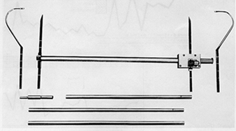
A stadiometer is a fixed anthropometer, generally used only for stature and frequently associated with a weight beam scale.
For transverse diameters a series of calipers may be used: the pelvimeter for measures up to 600 mm and the cephalometer up to 300 mm. The latter is particularly suitable for head measurements when used together with a sliding compass (figure 2).
Figure 2. A cephalometer together with a sliding compass

The foot-board is used for measuring the feet and the head-board provides cartesian co-ordinates of the head when oriented in the “Frankfort plane” (a horizontal plane passing through porion and orbitale landmarks of the head).The hand may be measured with a caliper, or with a special device composed of five sliding rulers.
Skinfold thickness is measured with a constant-pressure skinfold caliper generally with a pressure of 9.81 x 10⁴ Pa (the pressure imposed by a weight of 10 g on an area of 1 mm2).
For arcs and girths a narrow, flexible steel tape with flat section is used. Self-straightening steel tapes must be avoided.
Systems of variables
A system of anthropometric variables is a coherent set of body measurements to solve some specific problems.
In the field of ergonomics and safety, the main problem is fitting equipment and workspace to humans and tailoring clothes to the right size.
Equipment and workspace require mainly linear measures of limbs and body segments that can easily be calculated from landmark heights and diameters, whereas tailoring sizes are based mainly on arcs, girths and flexible tape lengths. Both systems may be combined according to need.
In any case, it is absolutely necessary to have a precise space reference for each measurement. The landmarks must, therefore, be linked by heights and diameters and every arc or girth must have a defined landmark reference. Heights and slopes must be indicated.
In a particular survey, the number of variables has to be limited to the minimum so as to avoid undue stress on the subject and operator.
A basic set of variables for workspace has been reduced to 33 measured variables (figure 3) plus 20 derived by a simple calculation. For a general-purpose military survey, Hertzberg and co-workers use 146 variables. For clothes and general biological purposes the Italian Fashion Board (Ente Italiano della Moda) uses a set of 32 general purpose variables and 28 technical ones. The German norm (DIN 61 516) of control body dimensions for clothes includes 12 variables. The recommendation of the International Organization for Standardization (ISO) for anthropometry includes a core list of 36 variables (see table 1). The International Data on Anthropometry tables published by the ILO list 19 body dimensions for the populations of 20 different regions of the world (Jürgens, Aune and Pieper 1990).
Figure 3. Basic set of anthropometric variables
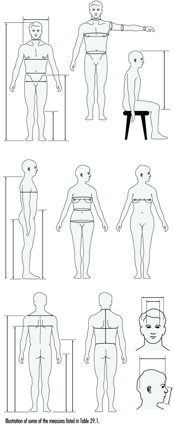
Table 1. Basic anthropometric core list
1.1 Forward reach (to hand grip with subject standing upright against a wall)
1.2 Stature (vertical distance from floor to head vertex)
1.3 Eye height (from floor to inner eye corner)
1.4 Shoulder height (from floor to acromion)
1.5 Elbow height (from floor to radial depression of elbow)
1.6 Crotch height (from floor to pubic bone)
1.7 Finger tip height (from floor to grip axis of fist)
1.8 Shoulder breadth (biacromial diameter)
1.9 Hip breadth, standing (the maximum distance across hips)
2.1 Sitting height (from seat to head vertex)
2.2 Eye height, sitting (from seat to inner corner of the eye)
2.3 Shoulder height, sitting (from seat to acromion)
2.4 Elbow height, sitting (from seat to lowest point of bent elbow)
2.5 Knee height (from foot-rest to the upper surface of thigh)
2.6 Lower leg length (height of sitting surface)
2.7 Forearm-hand length (from back of bent elbow to grip axis)
2.8 Body depth, sitting (seat depth)
2.9 Buttock-knee length (from knee-cap to rearmost point of buttock)
2.10 Elbow to elbow breadth (distance between lateral surface of the elbows)
2.11 Hip breadth, sitting (seat breadth)
3.1 Index finger breadth, proximal (at the joint between medial and proximal phalanges)
3.2 Index finger breadth, distal (at the joint between distal and medial phalanges)
3.3 Index finger length
3.4 Hand length (from tip of middle finger to styloid)
3.5 Handbreadth (at metacarpals)
3.6 Wrist circumference
4.1 Foot breadth
4.2 Foot length
5.1 Heat circumference (at glabella)
5.2 Sagittal arc (from glabella to inion)
5.3 Head length (from glabella to opisthocranion)
5.4 Head breadth (maximum above the ear)
5.5 Bitragion arc (over the head between the ears)
6.1 Waist circumference (at the umbilicus)
6.2 Tibial height (from the floor to the highest point on the antero-medial margin of the glenoid of the tibia)
6.3 Cervical height sitting (to the tip of the spinous process of the 7th cervical vertebra).
Source: Adapted from ISO/DP 7250 1980).
Precision and errors
The precision of living body dimensions must be considered in a stochastic manner because the human body is highly unpredictable, both as a static and as a dynamic structure.
A single individual may grow or change in muscularity and fatness; undergo skeletal changes as a consequence of aging, disease or accidents; or modify behavior or posture. Different subjects differ by proportions, not only by general dimensions. Tall stature subjects are not mere enlargements of short ones; constitutional types and somatotypes probably vary more than general dimensions.
The use of mannequins, particularly those representing the standard 5th, 50th and 95th percentiles for fitting trials may be highly misleading, if body variations in body proportions are not taken into consideration.
Errors result from misinterpretation of landmarks and incorrect use of instruments (personal error), imprecise or inexact instruments (instrumental error), or changes in subject posture (subject error—this latter may be due to difficulties of communication if the cultural or linguistic background of the subject differs from that of the operator).
Statistical treatment
Anthropometric data must be treated by statistical procedures, mainly in the field of inference methods applying univariate (mean, mode, percentiles, histograms, variance analysis, etc.), bivariate (correlation, regression) and multivariate (multiple correlation and regression, factor analysis, etc.) methods. Various graphical methods based on statistical applications have been devised to classify human types (anthropometrograms, morphosomatograms).
Sampling and survey
As anthropometric data cannot be collected for the whole population (except in the rare case of a particularly small population), sampling is generally necessary. A basically random sample should be the starting point of any anthropometric survey. To keep the number of measured subjects to a reasonable level it is generally necessary to have recourse to multiple-stage stratified sampling. This allows the most homogeneous subdivision of the population into a number of classes or strata.
The population may be subdivided by sex, age group, geographical area, social variables, physical activity and so on.
Survey forms have to be designed keeping in mind both measuring procedure and data treatment. An accurate ergonomic study of the measuring procedure should be made in order to reduce the operator’s fatigue and possible errors. For this reason, variables must be grouped according to the instrument used and ordered in sequence so as to reduce the number of body flexions the operator has to make.
To reduce the effect of personal error, the survey should be carried out by one operator. If more than one operator has to be used, training is necessary to assure the replicability of measurements.
Population anthropometrics
Disregarding the highly criticized concept of “race”, human populations are nevertheless highly variable in size of individuals and in size distribution. Generally human populations are not strictly Mendelian; they are commonly the result of admixture. Sometimes two or more populations, with different origins and adaptation, live together in the same area without interbreeding. This complicates the theoretical distribution of traits. From the anthropometric viewpoint, sexes are different populations. Populations of employees may not correspond exactly to the biological population of the same area as a consequence of possible aptitudinal selection or auto-selection due to job choice.
Populations from different areas may differ as a consequence of different adaptation conditions or biological and genetic structures.
When close fitting is important a survey on a random sample is necessary.
Fitting trials and regulation
The adaptation of workspace or equipment to the user may depend not only on the bodily dimensions, but also on such variables as tolerance of discomfort and nature of activities, clothing, tools and environmental conditions. A combination of a checklist of relevant factors, a simulator and a series of fitting trials using a sample of subjects chosen to represent the range of body sizes of the expected user population can be used.
The aim is to find tolerance ranges for all subjects. If the ranges overlap it is possible to select a narrower final range that is not outside the tolerance limits of any subject. If there is no overlap it will be necessary to make the structure adjustable or to provide it in different sizes. If more than two dimensions are adjustable a subject may not be able to decide which of the possible adjustments will fit him best.
Adjustability can be a complicated matter, especially when uncomfortable postures result in fatigue. Precise indications must, therefore, be given to the user who frequently knows little or nothing about his own anthropometric characteristics. In general, an accurate design should reduce the need for adjustment to the minimum. In any case, it should constantly be kept in mind what is involved is anthropometrics, not merely engineering.
Dynamic anthropometrics
Static anthropometrics may give wide information about movement if an adequate set of variables has been chosen. Nevertheless, when movements are complicated and a close fit with the industrial environment is desirable, as in most user-machine and human-vehicle interfaces, an exact survey of postures and movements is necessary. This may be done with suitable mock-ups that allow tracing of reach lines or by photography. In this case, a camera fitted with a telephoto lens and an anthropometric rod, placed in the sagittal plane of the subject, allows standardized photographs with little distortion of the image. Small labels on subjects’ articulations make the exact tracing of movements possible.
Another way of studying movements is to formalize postural changes according to a series of horizontal and vertical planes passing through the articulations. Again, using computerized human models with computer-aided design (CAD) systems is a feasible way to include dynamic anthropometrics in ergonomic workplace design.
Introduction and Concepts
Mechanistic toxicology is the study of how chemical or physical agents interact with living organisms to cause toxicity. Knowledge of the mechanism of toxicity of a substance enhances the ability to prevent toxicity and design more desirable chemicals; it constitutes the basis for therapy upon overexposure, and frequently enables a further understanding of fundamental biological processes. For purposes of this Encyclopaedia the emphasis will be placed on animals to predict human toxicity. Different areas of toxicology include mechanistic, descriptive, regulatory, forensic and environmental toxicology (Klaassen, Amdur and Doull 1991). All of these benefit from understanding the fundamental mechanisms of toxicity.
Why Understand Mechanisms of Toxicity?
Understanding the mechanism by which a substance causes toxicity enhances different areas of toxicology in different ways. Mechanistic understanding helps the governmental regulator to establish legally binding safe limits for human exposure. It helps toxicologists in recommending courses of action regarding clean-up or remediation of contaminated sites and, along with physical and chemical properties of the substance or mixture, can be used to select the degree of protective equipment required. Mechanistic knowledge is also useful in forming the basis for therapy and the design of new drugs for treatment of human disease. For the forensic toxicologist the mechanism of toxicity often provides insight as to how a chemical or physical agent can cause death or incapacitation.
If the mechanism of toxicity is understood, descriptive toxicology becomes useful in predicting the toxic effects of related chemicals. It is important to understand, however, that a lack of mechanistic information does not deter health professionals from protecting human health. Prudent decisions based on animal studies and human experience are used to establish safe exposure levels. Traditionally, a margin of safety was established by using the “no adverse effect level” or a “lowest adverse effect level” from animal studies (using repeated-exposure designs) and dividing that level by a factor of 100 for occupational exposure or 1,000 for other human environmental exposure. The success of this process is evident from the few incidents of adverse health effects attributed to chemical exposure in workers where appropriate exposure limits had been set and adhered to in the past. In addition, the human lifespan continues to increase, as does the quality of life. Overall the use of toxicity data has led to effective regulatory and voluntary control. Detailed knowledge of toxic mechanisms will enhance the predictability of newer risk models currently being developed and will result in continuous improvement.
Understanding environmental mechanisms is complex and presumes a knowledge of ecosystem disruption and homeostasis (balance). While not discussed in this article, an enhanced understanding of toxic mechanisms and their ultimate consequences in an ecosystem would help scientists to make prudent decisions regarding the handling of municipal and industrial waste material. Waste management is a growing area of research and will continue to be very important in the future.
Techniques for Studying Mechanisms of Toxicity
The majority of mechanistic studies start with a descriptive toxicological study in animals or clinical observations in humans. Ideally, animal studies include careful behavioural and clinical observations, careful biochemical examination of elements of the blood and urine for signs of adverse function of major biological systems in the body, and a post-mortem evaluation of all organ systems by microscopic examination to check for injury (see OECD test guidelines; EC directives on chemical evaluation; US EPA test rules; Japan chemicals regulations). This is analogous to a thorough human physical examination that would take place in a hospital over a two- to three-day time period except for the post-mortem examination.
Understanding mechanisms of toxicity is the art and science of observation, creativity in the selection of techniques to test various hypotheses, and innovative integration of signs and symptoms into a causal relationship. Mechanistic studies start with exposure, follow the time-related distribution and fate in the body (pharmacokinetics), and measure the resulting toxic effect at some level of the system and at some dose level. Different substances can act at different levels of the biological system in causing toxicity.
Exposure
The route of exposure in mechanistic studies is usually the same as for human exposure. Route is important because there can be effects that occur locally at the site of exposure in addition to systemic effects after the chemical has been absorbed into the blood and distributed throughout the body. A simple yet cogent example of a local effect would be irritation and eventual corrosion of the skin following application of strong acid or alkaline solutions designed for cleaning hard surfaces. Similarly, irritation and cellular death can occur in cells lining the nose and/or lungs following exposure to irritant vapours or gases such as oxides of nitrogen or ozone. (Both are constituents of air pollution, or smog). Following absorption of a chemical into blood through the skin, lungs or gastrointestinal tract, the concentration in any organ or tissue is controlled by many factors which determine the pharmacokinetics of the chemical in the body. The body has the ability to activate as well as detoxify various chemicals as noted below.
Role of Pharmacokinetics in Toxicity
Pharmacokinetics describes the time relationships for chemical absorption, distribution, metabolism (biochemical alterations in the body) and elimination or excretion from the body. Relative to mechanisms of toxicity, these pharmacokinetic variables can be very important and in some instances determine whether toxicity will or will not occur. For instance, if a material is not absorbed in a sufficient amount, systemic toxicity (inside the body) will not occur. Conversely, a highly reactive chemical that is detoxified quickly (seconds or minutes) by digestive or liver enzymes may not have the time to cause toxicity. Some polycyclic halogenated substances and mixtures as well as certain metals like lead would not cause significant toxicity if excretion were rapid; but accumulation to sufficiently high levels determines their toxicity since excretion is not rapid (sometimes measured in years). Fortunately, most chemicals do not have such long retention in the body. Accumulation of an innocuous material still would not induce toxicity. The rate of elimination from the body and detoxication is frequently referred to as the half-life of the chemical, which is the time for 50% of the chemical to be excreted or altered to a non-toxic form.
However, if a chemical accumulates in a particular cell or organ, that may signal a reason to further examine its potential toxicity in that organ. More recently, mathematical models have been developed to extrapolate pharmacokinetic variables from animals to humans. These pharmacokinetic models are extremely useful in generating hypotheses and testing whether the experimental animal may be a good representation for humans. Numerous chapters and texts have been written on this subject (Gehring et al. 1976; Reitz et al. 1987; Nolan et al. 1995). A simplified example of a physiological model is depicted in figure 1.
Figure 1. A simplified pharmacokinetic model
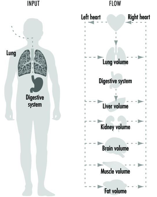
Different Levels and Systems Can Be Adversely Affected
Toxicity can be described at different biological levels. Injury can be evaluated in the whole person (or animal), the organ system, the cell or the molecule. Organ systems include the immune, respiratory, cardiovascular, renal, endocrine, digestive, muscolo-skeletal, blood, reproductive and central nervous systems. Some key organs include the liver, kidney, lung, brain, skin, eyes, heart, testes or ovaries, and other major organs. At the cellular/biochemical level, adverse effects include interference with normal protein function, endocrine receptor function, metabolic energy inhibition, or xenobiotic (foreign substance) enzyme inhibition or induction. Adverse effects at the molecular level include alteration of the normal function of DNA-RNA transcription, of specific cytoplasmic and nuclear receptor binding, and of genes or gene products. Ultimately, dysfunction in a major organ system is likely caused by a molecular alteration in a particular target cell within that organ. However, it is not always possible to trace a mechanism back to a molecular origin of causation, nor is it necessary. Intervention and therapy can be designed without a complete understanding of the molecular target. However, knowledge about the specific mechanism of toxicity increases the predictive value and accuracy of extrapolation to other chemicals. Figure 2 is a diagrammatic representation of the various levels where interference of normal physiological processes can be detected. The arrows indicate that the consequences to an individual can be determined from top down (exposure, pharmaco- kinetics to system/organ toxicity) or from bottom up (molecular change, cellular/biochemical effect to system/organ toxicity).
Figure 2. Reresentation of mechanisms of toxicity

Examples of Mechanisms of Toxicity
Mechanisms of toxicity can be straightforward or very complex. Frequently, there is a difference among the type of toxicity, the mechanism of toxicity, and the level of effect, related to whether the adverse effects are due to a single, acute high dose (like an accidental poisoning), or a lower-dose repeated exposure (from occupational or environmental exposure). Classically, for testing purposes, an acute, single high dose is given by direct intubation into the stomach of a rodent or exposure to an atmosphere of a gas or vapour for two to four hours, whichever best resembles the human exposure. The animals are observed over a two-week period following exposure and then the major external and internal organs are examined for injury. Repeated-dose testing ranges from months to years. For rodent species, two years is considered a chronic (lifetime) study sufficient to evaluate toxicity and carcinogenicity, whereas for non-human primates, two years would be considered a subchronic (less than lifetime) study to evaluate repeated dose toxicity. Following exposure a complete examination of all tissues, organs and fluids is conducted to determine any adverse effects.
Acute Toxicity Mechanisms
The following examples are specific to high-dose, acute effects which can lead to death or severe incapacitation. However, in some cases, intervention will result in transient and fully reversible effects. The dose or severity of exposure will determine the result.
Simple asphyxiants. The mechanism of toxicity for inert gases and some other non-reactive substances is lack of oxygen (anoxia). These chemicals, which cause deprivation of oxygen to the central nervous system (CNS), are termed simple asphyxiants. If a person enters a closed space that contains nitrogen without sufficient oxygen, immediate oxygen depletion occurs in the brain and leads to unconsciousness and eventual death if the person is not rapidly removed. In extreme cases (near zero oxygen) unconsciousness can occur in a few seconds. Rescue depends on rapid removal to an oxygenated environment. Survival with irreversible brain damage can occur from delayed rescue, due to the death of neurons, which cannot regenerate.
Chemical asphyxiants. Carbon monoxide (CO) competes with oxygen for binding to haemoglobin (in red blood cells) and therefore deprives tissues of oxygen for energy metabolism; cellular death can result. Intervention includes removal from the source of CO and treatment with oxygen. The direct use of oxygen is based on the toxic action of CO. Another potent chemical asphyxiant is cyanide. The cyanide ion interferes with cellular metabolism and utilization of oxygen for energy. Treatment with sodium nitrite causes a change in haemoglobin in red blood cells to methaemoglobin. Methaemoglobin has a greater binding affinity to the cyanide ion than does the cellular target of cyanide. Consequently, the methaemoglobin binds the cyanide and keeps the cyanide away from the target cells. This forms the basis for antidotal therapy.
Central nervous system (CNS) depressants. Acute toxicity is characterized by sedation or unconsciousness for a number of materials like solvents which are not reactive or which are transformed to reactive intermediates. It is hypothesized that sedation/anaesthesia is due to an interaction of the solvent with the membranes of cells in the CNS, which impairs their ability to transmit electrical and chemical signals. While sedation may seem a mild form of toxicity and was the basis for development of the early anaesthetics, “the dose still makes the poison”. If sufficient dose is administered by ingestion or inhalation the animal can die due to respiratory arrest. If anaesthetic death does not occur, this type of toxicity is usually readily reversible when the subject is removed from the environment or the chemical is redistributed or eliminated from the body.
Skin effects. Adverse effects to the skin can range from irritation to corrosion, depending on the substance encountered. Strong acids and alkaline solutions are incompatible with living tissue and are corrosive, causing chemical burns and possible scarring. Scarring is due to death of the dermal, deep skin cells responsible for regeneration. Lower concentrations may just cause irritation of the first layer of skin.
Another specific toxic mechanism of skin is that of chemical sensitization. As an example, sensitization occurs when 2,4-dinitrochlorobenzene binds with natural proteins in the skin and the immune system recognizes the altered protein-bound complex as a foreign material. In responding to this foreign material, the immune system activates special cells to eliminate the foreign substance by release of mediators (cytokines) which cause a rash or dermatitis (see “Immunotoxicology”). This is the same reaction of the immune system when exposure to poison ivy occurs. Immune sensitization is very specific to the particular chemical and takes at least two exposures before a response is elicited. The first exposure sensitizes (sets up the cells to recognize the chemical), and subsequent exposures trigger the immune system response. Removal from contact and symptomatic therapy with steroid-containing anti-inflammatory creams are usually effective in treating sensitized individuals. In serious or refractory cases a systemic acting immunosuppresant like prednisone is used in conjunction with topical treatment.
Lung sensitization. An immune sensitization response is elicited by toluene diisocyanate (TDI), but the target site is the lungs. TDI over-exposure in susceptible individuals causes lung oedema (fluid build-up), bronchial constriction and impaired breathing. This is a serious condition and requires removing the individual from potential subsequent exposures. Treatment is primarily symptomatic. Skin and lung sensitization follow a dose response. Exceeding the level set for occupational exposure can cause adverse effects.
Eye effects. Injury to the eye ranges from reddening of the outer layer (swimming-pool redness) to cataract formation of the cornea to damage to the iris (coloured part of the eye). Eye irritation tests are conducted when it is believed serious injury will not occur. Many of the mechanisms causing skin corrosion can also cause injury to the eyes. Materials corrosive to the skin, like strong acids (pH less than 2) and alkali (pH greater than 11.5), are not tested in the eyes of animals because most will cause corrosion and blindness due to a mechanism similar to that which causes skin corrosion. In addition, surface active agents like detergents and surfactants can cause eye injury ranging from irritation to corrosion. A group of materials that requires caution is the positively charged (cationic) surfactants, which can cause burns, permanent opacity of the cornea and vascularization (formation of blood vessels). Another chemical, dinitrophenol, has a specific effect of cataract formation. This appears to be related to concentration of this chemical in the eye, which is an example of pharmacokinetic distributional specificity.
While the listing above is far from exhaustive, it is designed to give the reader an appreciation for various acute toxicity mechanisms.
Subchronic and Chronic Toxicity Mechanisms
When given as a single high dose, some chemicals do not have the same mechanism of toxicity as when given repeatedly as a lower but still toxic dose. When a single high dose is given, there is always the possibility of exceeding the person’s ability to detoxify or excrete the chemical, and this can lead to a different toxic response than when lower repetitive doses are given. Alcohol is a good example. High doses of alcohol lead to primary central nervous system effects, while lower repetitive doses result in liver injury.
Anticholinesterase inhibition. Most organophosphate pesticides, for example, have little mammalian toxicity until they are metabolically activated, primarily in the liver. The primary mechanism of action of organophosphates is the inhibition of acetylcholinesterase (AChE) in the brain and peripheral nervous system. AChE is the normal enzyme that terminates the stimulation of the neurotransmitter acetylcholine. Slight inhibition of AChE over an extended period has not been associated with adverse effects. At high levels of exposure, inability to terminate this neuronal stimulation results in overstimulation of the cholinergic nervous system. Cholinergic overstimulation ultimately results in a host of symptoms, including respiratory arrest, followed by death if not treated. The primary treatment is the administration of atropine, which blocks the effects of acetylcholine, and the administration of pralidoxime chloride, which reactivates the inhibited AChE. Therefore, both the cause and the treatment of organophosphate toxicity are addressed by understanding the biochemical basis of toxicity.
Metabolic activation. Many chemicals, including carbon tetrachloride, chloroform, acetylaminofluorene, nitrosamines, and paraquat are metabolically activated to free radicals or other reactive intermediates which inhibit and interfere with normal cellular function. At high levels of exposure this results in cell death (see “Cellular injury and cellular death”). While the specific interactions and cellular targets remain unknown, the organ systems which have the capability to activate these chemicals, like the liver, kidney and lung, are all potential targets for injury. Specifically, particular cells within an organ have a greater or lesser capacity to activate or detoxify these intermediates, and this capacity determines the intracellular susceptibility within an organ. Metabolism is one reason why an understanding of pharmacokinetics, which describes these types of transformations and the distribution and elimination of these intermediates, is important in recognizing the mechanism of action of these chemicals.
Cancer mechanisms. Cancer is a multiplicity of diseases, and while the understanding of certain types of cancer is increasing rapidly due to the many molecular biological techniques that have been developed since 1980, there is still much to learn. However, it is clear that cancer development is a multi-stage process, and critical genes are key to different types of cancer. Alterations in DNA (somatic mutations) in a number of these critical genes can cause increased susceptibility or cancerous lesions (see “Genetic toxic- ology”). Exposure to natural chemicals (in cooked foods like beef and fish) or synthetic chemicals (like benzidine, used as a dye) or physical agents (ultraviolet light from the sun, radon from soil, gamma radiation from medical procedures or industrial activity) are all contributors to somatic gene mutations. However, there are natural and synthetic substances (such as anti-oxidants) and DNA repair processes which are protective and maintain homeostasis. It is clear that genetics is an important factor in cancer, since genetic disease syndromes such as xeroderma pigmentosum, where there is a lack of normal DNA repair, dramatically increase susceptibility to skin cancer from exposure to ultraviolet light from the sun.
Reproductive mechanisms. Similar to cancer, many mechanisms of reproductive and/or developmental toxicity are known, but much is to be learned. It is known that certain viruses (such as rubella), bacterial infections and drugs (such as thalidomide and vitamin A) will adversely affect development. Recently, work by Khera (1991), reviewed by Carney (1994), show good evidence that the abnormal developmental effects in animal tests with ethylene glycol are attributable to maternal metabolic acidic metabolites. This occurs when ethylene glycol is metabolized to acid metabolites including glycolic and oxalic acid. The subsequent effects on the placenta and foetus appear to be due to this metabolic toxication process.
Conclusion
The intent of this article is to give a perspective on several known mechanisms of toxicity and the need for future study. It is important to understand that mechanistic knowledge is not absolutely necessary to protect human or environmental health. This knowledge will enhance the professional’s ability to better predict and manage toxicity. The actual techniques used in elucidating any particular mechanism depend upon the collective knowledge of the scientists and the thinking of those who make decisions regarding human health.
Exposure Assessment
The assessment of exposures is a critical step in identifying workplace hazards through epidemiological investigation. The exposure assessment process may be subdivided into a series of activities. These include:
- compiling an inventory of potentially toxic agents and mixtures present in the targeted work environment
- determining how exposures occur and how likely they are to vary among employees
- selecting appropriate measures or indices for quantifying exposures
- collecting data that will enable study participants to be assigned qualitative or quantitative exposure values for each measure. Whenever possible, these activities should be carried out under the guidance of a qualified industrial hygienist.
Occupational health studies are often criticized because of inadequacies in the assessment of exposures. Inadequacies may lead to differential or non-differential misclassification of exposure and subsequent bias or loss of precision in the exposure-effect analyses. Efforts to improve the situation are evidenced by several recent international conferences and texts devoted to this topic (ACGIH 1991; Armstrong et al. 1992; Proceedings of the Conference on Retrospective Assessment of Occupational Exposures in Epidemiology 1995). Clearly, technical developments are providing new opportunities for advancing exposure assessment. These developments include improvements in analytical instrumentation, a better understanding of pharmacokinetic processes, and the discovery of new biomarkers of exposure. Because occupational health studies often depend on historic exposure information for which no specific monitoring would have been undertaken, the need for retrospective exposure assessment adds an additional dimension of complexity to these studies. However, improved standards for assessment and for ensuring the reliability of such assessments continue to be developed (Siemiatycki et al. 1986). Prospective exposure assessments, of course, can be more readily validated.
The term exposure refers to the concentration of an agent at the boundary between individual and environment. Exposure is normally presumed when an agent is known to be present in a work environment and there is a reasonable expectation of employee contact with that agent. Exposures may be expressed as an 8-hour time-weighted-average (TWA) concentration, which is a measure of exposure intensity that has been averaged over an 8-hour work shift. Peak concentrations are intensities averaged over shorter time periods such as 15 minutes. Cumulative exposure is a measure of the product of average intensity and duration (e.g., a mean 8-hour TWA concentration multiplied by years worked at that mean concentration). Depending on the nature of the study and the health outcomes of interest, evaluation of peak, average intensity, cumulative or lagged exposures may be desirable.
By way of contrast, dose refers to the deposition or absorption of an agent per unit time. Dose or daily intake of an agent may be estimated by combining environmental measurement data with standard assumptions regarding, among other factors, breathing rates and dermal penetration. Alternatively, intake may be estimated based on biomonitoring data. Dose ideally would be measured at the target organ of interest.
Important exposure assessment factors include:
- identification of the relevant agents
- determination of their presence and concentrations in appropriate environmental media (e.g., air, contact surfaces)
- assessment of the likely routes of entry (inhalation, skin absorption, ingestion), the time course of exposure (daily variation), and cumulative duration of exposure expressed in weeks, months or years
- evaluation of the effectiveness of engineering and personal controls (e.g., use of protective clothing and respiratory protection may mediate exposures) and, finally
- host and other considerations that may modulate target organ concentrations.
These include the physical level of work activity and the prior health status of individuals. Special care should be taken in assessing exposure to agents that are persistent or tend to bioaccumulate (e.g., certain metals, radionuclides or stable organic compounds). With these materials, internal body burdens may increase insidiously even when environmental concentrations appear to be low.
While the situation can be quite complex, often it is not. Certainly, many valuable contributions to identifying occupational hazards have come from studies using common-sense approaches to exposure assessment. Sources of information that can be helpful in identifying and categorizing exposures include:
- employee interviews
- employer personnel and production records (these include work records, job descriptions, facility and process histories, and chemical inventories)
- expert judgement
- industrial hygiene records (area, personal, and compliance monitoring, and surface wipe samples, together with health hazard or comprehensive survey reports)
- interviews with long-term or retired employees and
- biomonitoring data.
There are several advantages to categorizing individual exposures in as much detail as possible. Clearly, the informativeness of a study will be enhanced to the extent that the relevant exposures have been adequately described. Secondly, the credibility of the findings may be increased because the potential for confounding can be addressed more satisfactorily. For example, referents and exposed individuals will differ as to exposure status, but may also differ relative to other measured and unmeasured explanatory factors for the disease of interest. However, if an exposure gradient can be established within the study population, it is less likely that the same degree of confounding will persist within exposure subgroups, thus strengthening the overall study findings.
Job Exposure Matrices
One of the more practical and frequently used approaches to exposure assessment has been to estimate exposures indirectly on the basis of job titles. The use of job exposure matrices can be effective when complete work histories are available and there is a reasonable constancy in both the tasks and exposures associated with the jobs under study. On the broadest scale, standard industry and job title groupings have been devised from routinely collected census data or occupational data provided on death certificates. Unfortunately, the information maintained in these large record systems is often limited to the “current” or “usual” occupation. Furthermore, because the standard groupings do not take into account the conditions present in specific workplaces, they must usually be regarded as crude exposure surrogates.
For community- and registry-based case-control studies, a more detailed exposure assessment has been achieved by utilizing expert opinion to translate job history data obtained through personal interview into semi-quantitative evaluations of likely exposures to specific agents (Siemiatycki et al. 1986). Experts, such as chemists and industrial hygienists, are chosen to assist in the exposure evaluation because of their knowledge and familiarity with various industrial processes. By combining the detailed questionnaire data with knowledge of industrial processes, this approach has been helpful in characterizing exposure differences across work facilities.
The job-exposure matrix approach has also been employed successfully in industry- and company-specific studies (Gamble and Spirtas 1976). Individual job histories (a chronological listing of past department and job assignments for each employee) are often retained in company personnel files and, when available, provide a complete job history for the employees while they are working at that facility. These data may be expanded upon through personal interviews of the study participants. The next step is to inventory all job titles and department or work area designations used during the study period. These may easily range into the hundreds or even thousands within large, multi-process facilities or across companies within an industry, when production, maintenance, research, engineering, plant support services and administrative jobs are all considered over time (often several decades), allowing for changes in industrial processes. Data consolidation can be facilitated by creating a computer file of all work history records and then using edit routines to standardize job title terminology. Those jobs involving relatively homogeneous exposures can be combined to simplify the process of linking exposures to individual jobs. However, the grouping of jobs and work locations should be supported wherever possible by measurement data collected according to a sound sampling strategy.
Even with computerized work histories, retrospective linkage of exposure data to individuals can be a difficult task. Certainly, workplace conditions will be altered as technologies change, product demand shifts, and new regulations are put in place. There may also be changes in product formulations and seasonal production patterns in many industries. Permanent records may be kept regarding some changes. However, it is less likely that records will be retained regarding seasonal and other marginal process and production changes. Employees also may be trained to perform multiple jobs and then be rotated among jobs as production demands change. All of these circumstances add complexity to the exposure profiles of employees. Nevertheless, there are also work settings that have remained relatively unchanged for many years. In the final analysis, each work setting must be evaluated in its own right.
Ultimately, it will be necessary to summarize the worklife exposure history of each person in a study. Considerable influence on the final exposure-effect measures of risk has been demonstrated (Suarez-Almazor et al. 1992), and hence great care has to be exercised in selecting the most appropriate summary measure of exposure.
Industrial Hygiene—Environmental Measurement
Monitoring of work exposures is a fundamental ongoing activity in protecting employee health. Thus, industrial hygiene records may already exist at the time an epidemiological study is being planned. If so, these data should be reviewed to determine how well the target population has been covered, how many years of data are represented in the files, and how easily the measurements can be linked to jobs, work areas and individuals. These determinations will be helpful both in assessing the feasibility of the epidemiological study and in identifying data gaps that could be remedied with additional exposure sampling.
The issue of how best to link measurement data to specific jobs and individuals is a particularly important one. Area and breathing zone sampling may be helpful to industrial hygienists in identifying emission sources for corrective actions, but could be less useful in characterizing actual employee exposures unless careful time studies of employee work activities have been performed. For example, continuous area monitoring may identify excursion exposures at certain times in the day, but the question remains as to whether or not employees were in the work area at that time.
Personal sampling data generally provide more accurate estimates of employee exposure as long as the sampling is carried out under representative conditions, the use of personal protective gear is properly taken into account, and the job tasks and process conditions are relatively constant from day to day. Personal samples may be readily linked to the individual employee through the use of personal identifiers. These data may be generalized to other employees in the same jobs and to other time periods as warranted. However, based on their own experience, Rappaport et al. (1993) have cautioned that exposure concentrations may be highly variable even among employees assigned to what are considered homogeneous exposure groups. Again, expert judgement is needed in deciding whether or not homogeneous exposure groups can be presumed.
Researchers have successfully combined a job-exposure matrix approach with utilization of environmental measurement data to estimate exposures within the cells of the matrix. When measurement data are found to be lacking, it may be possible to fill in data gaps through the use of exposure modelling. Generally, this involves developing a model for relating environmental concentrations to more easily assessed determinants of exposure concentrations (e.g., production volumes, physical characteristics of the facility including the use of exhaust ventilation systems, agent volatility and nature of the work activity). The model is constructed for work settings with known environmental concentrations and then used to estimate concentrations in similar work settings lacking measurement data but having information on such parameters as constituent ingredients and production volumes. This approach may be particularly helpful for the retrospective estimation of exposures.
Another important assessment issue is the handling of exposure to mixtures. First, from an analytic viewpoint, separate detection of chemically related compounds and elimination of interferences from other substances present in the sample may not be within the capability of the analytic procedure. The various limitations in the analytic procedures used to provide measurement data need to be evaluated and the study objectives modified accordingly. Secondly, it may be that certain agents are almost always used together and hence occur in approximately the same relative proportions throughout the work environment under study. In this situation, internal statistical analyses per se will not be useful in distinguishing whether or not effects are due to one or the other agents or due to a combination of the agents. Such judgements would only be possible based on review of external studies in which the same agent combinations had not occurred. Finally, in situations where different materials are used interchangeably depending on product specifications (e.g., the use of different colourants to obtain desired colour contrasts), it may be impossible to attribute effects to any specific agent.
Biological Monitoring
Biomarkers are molecular, biochemical or cellular alterations that can be measured in biological media such as human tissue, cells or fluids. A primary reason for developing biomarkers of exposure is to provide an estimate of internal dose for a particular agent. This approach is especially useful when multiple routes of exposure are likely (e.g., inhalation and skin absorption), when protective gear is worn intermittently, or when the conditions of exposure are unpredictable. Biomonitoring can be especially advantageous when the agents of interest are known to have relatively long biological half-lives. From a statistical perspective, an advantage of biological monitoring over air monitoring may be seen with agents having a half-life as short as ten hours, depending upon the degree of environmental variability (Droz and Wu 1991). The exceedingly long half-lives of materials such as chlorinated dioxins (measured in years) make these compounds ideal candidates for biological monitoring. As with analytical methods for measuring air concentrations, one must be aware of potential interferences. For example, before utilizing a particular metabolite as a biomarker, it should be determined whether or not other common substances, such as those contained in certain medications and in cigarette smoke, could be metabolized to the same end point. In general, basic knowledge of the pharmacokinetics of an agent is needed before biological monitoring is utilized as a basis for exposure assessment.
The most frequent points of measurement include alveolar air, urine and blood. Alveolar air samples may be helpful in characterizing high short-term solvent exposures that have occurred within minutes or hours of when the sample was collected. Urinary samples are typically collected to determine excretion rates for metabolites of the compound of interest. Blood samples may be collected for direct measurement of the compound, for measurement of metabolites, or for determination of protein or DNA adducts (e.g., albumin or haemoglobin adducts, and DNA adducts in circulating lymphocytes). Accessible tissue cells, such as epithelial cells from the buccal area of the mouth, may also be sampled for identification of DNA adducts.
Determination of cholinesterase activity in red blood cells and plasma exemplifies the use of biochemical alterations as a measure of exposure. Organophosphorus pesticides inhibit cholinesterase activity and hence measurement of that activity before and after likely exposure to these compounds can be a useful indicator of exposure intensity. However, as one progresses along the spectrum of biological alterations, it becomes more difficult to distinguish between biomarkers of exposure and those of effect. In general, effect measures tend to be non-specific for the substance of interest and, therefore, other potential explanations of the effect may need to be assessed in order to support using that parameter as an exposure measure. Exposure measures should either be directly tied to the agent of interest or there should be a sound basis for linking any indirect measure to the agent. Despite these qualifications, biological monitoring holds much promise as a means for improving exposure assessment in support of epidemiological studies.
Conclusions
In making comparisons in occupational epidemiology studies, the need is to have a group of workers with exposure to compare against a group of workers without exposure. Such distinctions are crude, but can be helpful in identifying problem areas. Clearly, however, the more refined the measure of exposure, the more useful will be the study, specifically in terms of its ability to identify and develop appropriately targeted intervention programmes.
Muscular Work
Muscular Work in Occupational Activities
In industrialized countries around 20% of workers are still employed in jobs requiring muscular effort (Rutenfranz et al. 1990). The number of conventional heavy physical jobs has decreased, but, on the other hand, many jobs have become more static, asymmetrical and stationary. In developing countries, muscular work of all forms is still very common.
Muscular work in occupational activities can be roughly divided into four groups: heavy dynamic muscle work, manual materials handling, static work and repetitive work. Heavy dynamic work tasks are found in forestry, agriculture and the construction industry, for example. Materials handling is common, for example, in nursing, transportation and warehousing, while static loads exist in office work, the electronics industry and in repair and maintenance tasks. Repetitive work tasks can be found in the food and wood-processing industries, for example.
It is important to note that manual materials handling and repetitive work are basically either dynamic or static muscular work, or a combination of these two.
Physiology of Muscular Work
Dynamic muscular work
In dynamic work, active skeletal muscles contract and relax rhythmically. The blood flow to the muscles is increased to match metabolic needs. The increased blood flow is achieved through increased pumping of the heart (cardiac output), decreased blood flow to inactive areas, such as kidneys and liver, and increased number of open blood vessels in the working musculature. Heart rate, blood pressure, and oxygen extraction in the muscles increase linearly in relation to working intensity. Also, pulmonary ventilation is heightened owing to deeper breathing and increased breathing frequency. The purpose of activating the whole cardio-respiratory system is to enhance oxygen delivery to the active muscles. The level of oxygen consumption measured during heavy dynamic muscle work indicates the intensity of the work. The maximum oxygen consumption (VO2max) indicates the person’s maximum capacity for aerobic work. Oxygen consumption values can be translated to energy expenditure (1 litre of oxygen consumption per minute corresponds to approximately 5 kcal/min or 21 kJ/min).
In the case of dynamic work, when the active muscle mass is smaller (as in the arms), maximum working capacity and peak oxygen consumption are smaller than in dynamic work with large muscles. At the same external work output, dynamic work with small muscles elicits higher cardio-respiratory responses (e.g., heart rate, blood pressure) than work with large muscles (figure 1).
Figure 1. Static versus dynamic work
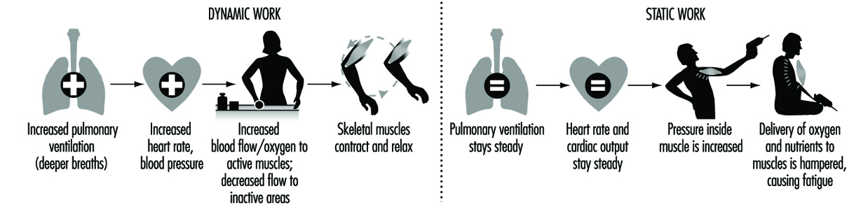
Static muscle work
In static work, muscle contraction does not produce visible movement, as, for example, in a limb. Static work increases the pressure inside the muscle, which together with the mechanical compression occludes blood circulation partially or totally. The delivery of nutrients and oxygen to the muscle and the removal of metabolic end-products from the muscle are hampered. Thus, in static work, muscles become fatigued more easily than in dynamic work.
The most prominent circulatory feature of static work is a rise in blood pressure. Heart rate and cardiac output do not change much. Above a certain intensity of effort, blood pressure increases in direct relation to the intensity and the duration of the effort. Furthermore, at the same relative intensity of effort, static work with large muscle groups produces a greater blood pressure response than does work with smaller muscles. (See figure 2)
Figure 2. The expanded stress-strain model modified from Rohmert (1984)

In principle, the regulation of ventilation and circulation in static work is similar to that in dynamic work, but the metabolic signals from the muscles are stronger, and induce a different response pattern.
Consequences of Muscular Overload in Occupational Activities
The degree of physical strain a worker experiences in muscular work depends on the size of the working muscle mass, the type of muscular contractions (static, dynamic), the intensity of contractions, and individual characteristics.
When muscular workload does not exceed the worker’s physical capacities, the body will adapt to the load and recovery is quick when the work is stopped. If the muscular load is too high, fatigue will ensue, working capacity is reduced, and recovery slows down. Peak loads or prolonged overload may result in organ damage (in the form of occupational or work-related diseases). On the other hand, muscular work of certain intensity, frequency, and duration may also result in training effects, as, on the other hand, excessively low muscular demands may cause detraining effects. These relationships are represented by the so-called expanded stress-strain concept developed by Rohmert (1984) (figure 3).
Figure 3. Analysis of acceptable workloads
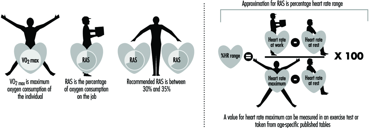
In general, there is little epidemiological evidence that muscular overload is a risk factor for diseases. However, poor health, disability and subjective overload at work converge in physically demanding jobs, especially with older workers. Furthermore, many risk factors for work-related musculoskeletal diseases are connected to different aspects of muscular workload, such as the exertion of strength, poor working postures, lifting and sudden peak loads.
One of the aims of ergonomics has been to determine acceptable limits for muscular workloads which could be applied for the prevention of fatigue and disorders. Whereas the prevention of chronic effects is the focus of epidemiology, work physiology deals mostly with short-term effects, that is, fatigue in work tasks or during a work day.
Acceptable Workload in Heavy Dynamic Muscular Work
The assessment of acceptable workload in dynamic work tasks has traditionally been based on measurements of oxygen consumption (or, correspondingly, energy expenditure). Oxygen consumption can be measured with relative ease in the field with portable devices (e.g., Douglas bag, Max Planck respirometer, Oxylog, Cosmed), or it can be estimated from heart rate recordings, which can be made reliably at the workplace, for example, with the SportTester device. The use of heart rate in the estimation of oxygen consumption requires that it be individually calibrated against measured oxygen consumption in a standard work mode in the laboratory, i.e., the investigator must know the oxygen consumption of the individual subject at a given heart rate. Heart rate recordings should be treated with caution because they are also affected by such factors as physical fitness, environmental temperature, psychological factors and size of active muscle mass. Thus, heart rate measurements can lead to overestimates of oxygen consumption in the same way that oxygen consumption values can give rise to underestimates of global physiological strain by reflecting only energy requirements.
Relative aerobic strain (RAS) is defined as the fraction (expressed as a percentage) of a worker’s oxygen consumption measured on the job relative to his or her VO2max measured in the laboratory. If only heart rate measurements are available, a close approximation to RAS can be made by calculating a value for percentage heart rate range (% HR range) with the so-called Karvonen formula as in figure 3.
VO2max is usually measured on a bicycle ergometer or treadmill, for which the mechanical efficiency is high (20-25%). When the active muscle mass is smaller or the static component is higher, VO2max and mechanical efficiency will be smaller than in the case of exercise with large muscle groups. For example, it has been found that in the sorting of postal parcels the VO2max of workers was only 65% of the maximum measured on a bicycle ergometer, and the mechanical efficiency of the task was less than 1%. When guidelines are based on oxygen consumption, the test mode in the maximal test should be as close as possible to the real task. This goal, however, is difficult to achieve.
According to Åstrand’s (1960) classical study, RAS should not exceed 50% during an eight-hour working day. In her experiments, at a 50% workload, body weight decreased, heart rate did not reach steady state and subjective discomfort increased during the day. She recommended a 50% RAS limit for both men and women. Later on she found that construction workers spontaneously chose an average RAS level of 40% (range 25-55%) during a working day. Several more recent studies have indicated that the acceptable RAS is lower than 50%. Most authors recommend 30-35% as an acceptable RAS level for the entire working day.
Originally, the acceptable RAS levels were developed for pure dynamic muscle work, which rarely occurs in real working life. It may happen that acceptable RAS levels are not exceeded, for example, in a lifting task, but the local load on the back may greatly exceed acceptable levels. Despite its limitations, RAS determination has been widely used in the assessment of physical strain in different jobs.
In addition to the measurement or estimation of oxygen consumption, other useful physiological field methods are also available for the quantification of physical stress or strain in heavy dynamic work. Observational techniques can be used in the estimation of energy expenditure (e.g., with the aid of the Edholm scale) (Edholm 1966). Rating of perceived exertion (RPE) indicates the subjective accumulation of fatigue. New ambulatory blood pressure monitoring systems allow more detailed analyses of circulatory responses.
Acceptable Workload in Manual Materials Handling
Manual materials handling includes such work tasks as lifting, carrying, pushing and pulling of various external loads. Most of the research in this area has focused on low back problems in lifting tasks, especially from the biomechanical point of view.
A RAS level of 20-35% has been recommended for lifting tasks, when the task is compared to an individual maximum oxygen consumption obtained from a bicycle ergometer test.
Recommendations for a maximum permissible heart rate are either absolute or related to the resting heart rate. The absolute values for men and women are 90-112 beats per minute in continuous manual materials handling. These values are about the same as the recommended values for the increase in heart rate above resting levels, that is, 30 to 35 beats per minute. These recommendations are also valid for heavy dynamic muscle work for young and healthy men and women. However, as mentioned previously, heart rate data should be treated with caution, because it is also affected by other factors than muscle work.
The guidelines for acceptable workload for manual materials handling based on biomechanical analyses comprise several factors, such as weight of the load, handling frequency, lifting height, distance of the load from the body and physical characteristics of the person.
In one large-scale field study (Louhevaara, Hakola and Ollila 1990) it was found that healthy male workers could handle postal parcels weighing 4 to 5 kilograms during a shift without any signs of objective or subjective fatigue. Most of the handling occurred below shoulder level, the average handling frequency was less than 8 parcels per minute and the total number of parcels was less than 1,500 per shift. The mean heart rate of the workers was 101 beats per minute and their mean oxygen consumption 1.0 l/min, which corresponded to 31% RAS as related to bicycle maximum.
Observations of working postures and use of force carried out for example according to OWAS method (Karhu, Kansi and Kuorinka 1977), ratings of perceived exertion and ambulatory blood pressure recordings are also suitable methods for stress and strain assessments in manual materials handling. Electromyography can be used to assess local strain responses, for example in arm and back muscles.
Acceptable Workload for Static Muscular Work
Static muscular work is required chiefly in maintaining working postures. The endurance time of static contraction is exponentially dependent on the relative force of contraction. This means, for example, that when the static contraction requires 20% of the maximum force, the endurance time is 5 to 7 minutes, and when the relative force is 50%, the endurance time is about 1 minute.
Older studies indicated that no fatigue will be developed when the relative force is below 15% of the maximum force. However, more recent studies have indicated that the acceptable relative force is specific to the muscle or muscle group, and is 2 to 5% of the maximum static strength. These force limits are, however, difficult to use in practical work situations because they require electromyographic recordings.
For the practitioner, fewer field methods are available for the quantification of strain in static work. Some observational methods (e.g., the OWAS method) exist to analyse the proportion of poor working postures, that is, postures deviating from normal middle positions of the main joints. Blood pressure measurements and ratings of perceived exertion may be useful, whereas heart rate is not so applicable.
Acceptable Workload in Repetitive Work
Repetitive work with small muscle groups resembles static muscle work from the point of view of circulatory and metabolic responses. Typically, in repetitive work muscles contract over 30 times per minute. When the relative force of contraction exceeds 10% of the maximum force, endurance time and muscle force start to decrease. However, there is wide individual variation in endurance times. For example, the endurance time varies between two to fifty minutes when the muscle contracts 90 to 110 times per minute at a relative force level of 10 to 20% (Laurig 1974).
It is very difficult to set any definitive criteria for repetitive work, because even very light levels of work (as with the use of a microcomputer mouse) may cause increases in intramuscular pressure, which may sometimes lead to swelling of muscle fibres, pain and reduction in muscle strength.
Repetitive and static muscle work will cause fatigue and reduced work capacity at very low relative force levels. Therefore, ergonomic interventions should aim to minimize the number of repetitive movements and static contractions as far as possible. Very few field methods are available for strain assessment in repetitive work.
Prevention of Muscular Overload
Relatively little epidemiological evidence exists to show that muscular load is harmful to health. However, work physiological and ergonomic studies indicate that muscular overload results in fatigue (i.e., decrease in work capacity) and may reduce productivity and quality of work.
The prevention of muscular overload may be directed to the work content, the work environment and the worker. The load can be adjusted by technical means, which focus on the work environment, tools, and/or the working methods. The fastest way to regulate muscular workload is to increase the flexibility of working time on an individual basis. This means designing work-rest regimens which take into account the workload and the needs and capacities of the individual worker.
Static and repetitive muscular work should be kept at a minimum. Occasional heavy dynamic work phases may be useful for the maintenance of endurance type physical fitness. Probably, the most useful form of physical activity that can be incorporated into a working day is brisk walking or stair climbing.
Prevention of muscular overload, however, is very difficult if a worker’s physical fitness or working skills are poor. Appropriate training will improve working skills and may reduce muscular loads at work. Also, regular physical exercise during work or leisure time will increase the muscular and cardio-respiratory capacities of the worker.
Cellular Injury and Cellular Death
Virtually all of medicine is devoted to either preventing cell death, in diseases such as myocardial infarction, stroke, trauma and shock, or causing it, as in the case of infectious diseases and cancer. It is, therefore, essential to understand the nature and mechanisms involved. Cell death has been classified as “accidental”, that is, caused by toxic agents, ischaemia and so on, or “programmed”, as occurs during embryological development, including formation of digits, and resorption of the tadpole tail.
Cell injury and cell death are, therefore, important both in physiology and in pathophysiology. Physiological cell death is extremely important during embryogenesis and embryonic development. The study of cell death during development has led to important and new information on the molecular genetics involved, especially through the study of development in invertebrate animals. In these animals, the precise location and the significance of cells that are destined to undergo cell death have been carefully studied and, with the use of classic mutagenesis techniques, several involved genes have now been identified. In adult organs, the balance between cell death and cell proliferation controls organ size. In some organs, such as the skin and the intestine, there is a continual turnover of cells. In the skin, for example, cells differentiate as they reach the surface, and finally undergo terminal differentiation and cell death as keratinization proceeds with the formation of crosslinked envelopes.
Many classes of toxic chemicals are capable of inducing acute cell injury followed by death. These include anoxia and ischaemia and their chemical analogues such as potassium cyanide; chemical carcinogens, which form electrophiles that covalently bind to proteins in nucleic acids; oxidant chemicals, resulting in free radical formation and oxidant injury; activation of complement; and a variety of calcium ionophores. Cell death is also an important component of chemical carcinogenesis; many complete chemical carcinogens, at carcinogenic doses, produce acute necrosis and inflammation followed by regeneration and preneoplasia.
Definitions
Cell injury
Cell injury is defined as an event or stimulus, such as a toxic chemical, that perturbs the normal homeostasis of the cell, thus causing a number of events to occur (figure 1). The principal targets of lethal injury illustrated are inhibition of ATP synthesis, disruption of plasma membrane integrity or withdrawal of essential growth factors.
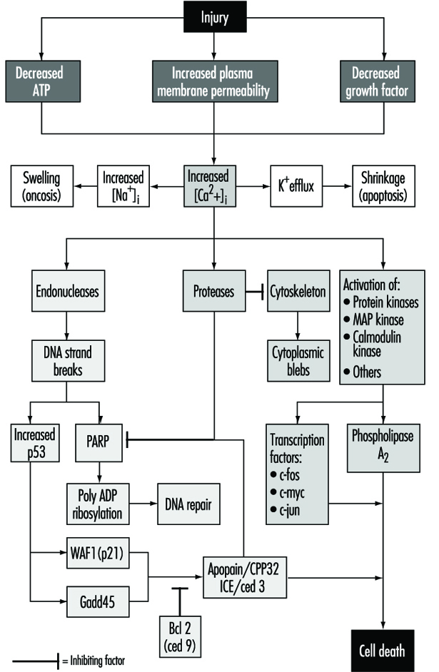
Lethal injuries result in the death of a cell after a variable period of time, depending on temperature, cell type and the stimulus; or they can be sublethal or chronic—that is, the injury results in an altered homeostatic state which, though abnormal, does not result in cell death (Trump and Arstila 1971; Trump and Berezesky 1992; Trump and Berezesky 1995; Trump, Berezesky and Osornio-Vargas 1981). In the case of a lethal injury, there is a phase prior to the time of cell death
during this time, the cell will recover; however, after a particular point in time (the “point of no return” or point of cell death), the removal of the injury does not result in recovery but instead the cell undergoes degradation and hydrolysis, ultimately reaching physical-chemical equilibrium with the environment. This is the phase known as necrosis. During the prelethal phase, several principal types of change occur, depending on the cell and the type of injury. These are known as apoptosis and oncosis.
Apoptosis
Apoptosis is derived from the Greek words apo, meaning away from, and ptosis, meaning to fall. The term falling away from is derived from the fact that, during this type of prelethal change, the cells shrink and undergo marked blebbing at the periphery. The blebs then detach and float away. Apoptosis occurs in a variety of cell types following various types of toxic injury (Wyllie, Kerr and Currie 1980). It is especially prominent in lymphocytes, where it is the predominant mechanism for turnover of lymphocyte clones. The resulting fragments result in the basophilic bodies seen within macrophages in lymph nodes. In other organs, apoptosis typically occurs in single cells which are rapidly cleared away before and following death by phagocytosis of the fragments by adjacent parenchymal cells or by macrophages. Apoptosis occurring in single cells with subsequent phagocytosis typically does not result in inflammation. Prior to death, apoptotic cells show a very dense cytosol with normal or condensed mitochondria. The endoplasmic reticulum (ER) is normal or only slightly dilated. The nuclear chromatin is markedly clumped along the nuclear envelope and around the nucleolus. The nuclear contour is also irregular and nuclear fragmentation occurs. The chromatin conden- sation is associated with DNA fragmentation which, in many instances, occurs between nucleosomes, giving a characteristic ladder appearance on electrophoresis.
In apoptosis, increased [Ca2+]i may stimulate K+ efflux resulting in cell shrinkage, which probably requires ATP. Injuries that totally inhibit ATP synthesis, therefore, are more likely to result in apoptosis. A sustained increase of [Ca2+]i has a number of deleterious effects including activation of proteases, endonucleases, and phospholipases. Endonuclease activation results in single and double DNA strand breaks which, in turn, stimulate increased levels of p53 and in poly-ADP ribosylation, and of nuclear proteins which are essential in DNA repair. Activation of proteases modifies a number of substrates including actin and related proteins leading to bleb formation. Another important substrate is poly(ADP-ribose) polymerase (PARP), which inhibits DNA repair. Increased [Ca2+]i is also associated with activation of a number of protein kinases, such as MAP kinase, calmodulin kinase and others. Such kinases are involved in activation of transcription factors which initiate transcription of immediate-early genes, for example, c-fos, c-jun and c-myc, and in activation of phospholipase A2 which results in permeabilization of the plasma membrane and of intracellular membranes such as the inner membrane of mitochondria.
Oncosis
Oncosis, derived from the Greek word onkos, to swell, is so named because in this type of prelethal change the cell begins to swell almost immediately following the injury (Majno and Joris 1995). The reason for the swelling is an increase in cations in the water within the cell. The principal cation responsible is sodium, which is normally regulated to maintain cell volume. However, in the absence of ATP or if Na-ATPase of the plasmalemma is inhibited, volume control is lost because of intracellular protein, and sodium in the water continuing to increase. Among the early events in oncosis are, therefore, increased [Na+]i which leads to cellular swelling and increased [Ca2+]i resulting either from influx from the extracellular space or release from intracellular stores. This results in swelling of the cytosol, swelling of the endoplasmic reticulum and Golgi apparatus, and the formation of watery blebs around the cell surface. The mitochondria initially undergo condensation, but later they too show high-amplitude swelling because of damage to the inner mitochondrial membrane. In this type of prelethal change, the chromatin undergoes condensation and ultimately degradation; however, the characteristic ladder pattern of apoptosis is not seen.
Necrosis
Necrosis refers to the series of changes that occur following cell death when the cell is converted to debris which is typically removed by the inflammatory response. Two types can be distinguished: oncotic necrosis and apoptotic necrosis. Oncotic necrosis typically occurs in large zones, for example, in a myocardial infarct or regionally in an organ after chemical toxicity, such as the renal proximal tubule following administration of HgCl2. Broad zones of an organ are involved and the necrotic cells rapidly incite an inflammatory reaction, first acute and then chronic. In the event that the organism survives, in many organs necrosis is followed by clearing away of the dead cells and regeneration, for example, in the liver or kidney following chemical toxicity. In contrast, apoptotic necrosis typically occurs on a single cell basis and the necrotic debris is formed within the phagocytes of macrophages or adjacent parenchymal cells. The earliest characteristics of necrotic cells include interruptions in plasma membrane continuity and the appearance of flocculent densities, representing denatured proteins within the mitochondrial matrix. In some forms of injury that do not initially interfere with mitochondrial calcium accumulation, calcium phosphate deposits can be seen within the mitochondria. Other membrane systems are similarly fragmenting, such as the ER, the lysosomes and the Golgi apparatus. Ultimately, the nuclear chromatin undergoes lysis, resulting from attack by lysosomal hydrolases. Following cell death, lysosomal hydrolases play an important part in clearing away debris with cathepsins, nucleolases and lipases since these have an acid pH optimum and can survive the low pH of necrotic cells while other cellular enzymes are denatured and inactivated.
Mechanisms
Initial stimulus
In the case of lethal injuries, the most common initial interactions resulting in injury leading to cell death are interference with energy metabolism, such as anoxia, ischaemia or inhibitors of respiration, and glycolysis such as potassium cyanide, carbon monoxide, iodo-acetate, and so on. As mentioned above, high doses of compounds that inhibit energy metabolism typically result in oncosis. The other common type of initial injury resulting in acute cell death is modification of the function of the plasma membrane (Trump and Arstila 1971; Trump, Berezesky and Osornio-Vargas 1981). This can either be direct damage and permeabilization, as in the case of trauma or activation of the C5b-C9 complex of complement, mechanical damage to the cell membrane or inhibition of the sodium-potassium (Na+-K+) pump with glycosides such as ouabain. Calcium ionophores such as ionomycin or A23187, which rapidly carry [Ca2+] down the gradient into the cell, also cause acute lethal injury. In some cases, the pattern in the prelethal change is apoptosis; in others, it is oncosis.
Signalling pathways
With many types of injury, mitochondrial respiration and oxidative phosphorylation are rapidly affected. In some cells, this stimulates anaerobic glycolysis, which is capable of maintaining ATP, but with many injuries this is inhibited. The lack of ATP results in failure to energize a number of important homeostatic processes, in particular, control of intracellular ion homeostasis (Trump and Berezesky 1992; Trump, Berezesky and Osornio-Vargas 1981). This results in rapid increases of [Ca2+]i, and increased [Na+] and [Cl-] results in cell swelling. Increases in [Ca2+]i result in the activation of a number of other signalling mechanisms discussed below, including a series of kinases, which can result in increased immediate early gene transcription. Increased [Ca2+]i also modifies cytoskeletal function, in part resulting in bleb formation and in the activation of endonucleases, proteases and phospholipases. These seem to trigger many of the important effects discussed above, such as membrane damage through protease and lipase activation, direct degradation of DNA from endonuclease activation, and activation of kinases such as MAP kinase and calmodulin kinase, which act as transcription factors.
Through extensive work on development in the invertebrate C. elegans and Drosophila, as well as human and animal cells, a series of pro-death genes have been identified. Some of these invertebrate genes have been found to have mammalian counterparts. For example, the ced-3 gene, which is essential for programmed cell death in C. elegans, has protease activity and a strong homology with the mammalian interleukin converting enzyme (ICE). A closely related gene called apopain or prICE has recently been identified with even closer homology (Nicholson et al. 1995). In Drosophila, the reaper gene seems to be involved in a signal that leads to programmed cell death. Other pro-death genes include the Fas membrane protein and the important tumour-suppressor gene, p53, which is widely conserved. p53 is induced at the protein level following DNA damage and when phosphorylated acts as a transcription factor for other genes such as gadd45 and waf-1, which are involved in cell death signalling. Other immediate early genes such as c-fos, c-jun, and c-myc also seem to be involved in some systems.
At the same time, there are anti-death genes which appear to counteract the pro-death genes. The first of these to be identified was ced-9 from C. elegans, which is homologous to bcl-2 in humans. These genes act in an as yet unknown way to prevent cell killing by either genetic or chemical toxins. Some recent evidence indicates that bcl-2 may act as an antioxidant. Currently, there is much effort underway to develop an understanding of the genes involved and to develop ways to activate or inhibit these genes, depending on the situation.
Summary Worklife Exposure Measures
Researchers are fortunate when they have at their disposal a detailed chronology of the worklife experience of workers that provides an historic review of jobs they have held over time. For these workers a job exposure matrix can then be set up that allows each and every job change that a worker has gone through to be associated with specific exposure information.
Detailed exposure histories must be summarized for analysis purposes in order to determine whether patterns are evident that could be related to health and safety issues in the workplace. We can visualize a list of, say, 20 job changes that a worker had experienced in his or her working lifetime. There are then several alternative ways in which the exposure details (for each of the 20 job changes in this example) can be summarized, taking duration and/or concentration/dose/grade of exposure into account.
It is important to note, however, that different conclusions from a study could be reached depending on the method selected (Suarez-Almazor et al. 1992). An example of five summary worklife exposure measures is shown in table 1.
Table 1. Formulae and dimensions or units of the five selected summary measures of worklife exposure
|
Exposure measure |
Formula |
Dimensions/Units |
|
Cumulative exposure index (CEI) |
Σ (grade x time exposed) |
grade and time |
|
Mean grade (MG) |
Σ (grade x time exposed)/total time exposed |
grade |
|
Highest grade ever (HG) |
highest grade to which exposed for ≥ 7 days |
grade |
|
Time-weighted average (TWA) grade |
Σ (grade x time exposed)/total time employed |
grade |
|
Total time exposed (TTE) |
Σ time exposed |
time |
Adapted from Suarez-Almazor et al. 1992.
Cumulative exposure index. The cumulative exposure index (CEI) is equivalent to “dose” in toxicological studies and represents the sum, over a working lifetime, of the products of exposure grade and exposure duration for each successive job title. It includes time in its units.
Mean grade. The mean grade (MG) cumulates the products of exposure grade and exposure duration for each successive job title (i.e., the CEI) and divides by the total time exposed at any grade greater than zero. MG is independent of time in its units; the summary measure for a person exposed for a long period at a high concentration will be similar to that for a person exposed for a short period at a high concentration. Within any matched set in a case-control design, MG is an average grade of exposure per unit of time exposed. It is an average grade for the time actually exposed to the agent under consideration.
Highest grade ever. The highest grade ever (HG) is determined from scanning the work history for the highest grade assignment in the period of observation to which the worker was exposed for at least seven days. The HG could misrepresent a person’s worklife exposure because, by its very formulation, it is based on a maximizing rather than on an averaging procedure and is therefore independent of duration of exposure in its units.
Time-weighted average grade. The time-weighted average (TWA) grade is the cumulative exposure index (CEI) divided by the total time employed. Within any matched set in a case-control design, the TWA grade averages over total time employed. It differs from MG, which averages only over the total time actually exposed. Thus, TWA grade can be viewed as an average exposure per unit of time in the full term of employment regardless of exposure per se.
Total time exposed. The total time exposed (TTE) accumulates all time periods associated with exposure in units of time. TTE has appeal for its simplicity. However, it is well accepted that health effects must be related not only to duration of chemical exposure, but also to the intensity of that exposure (i.e., the concentration or grade).
Clearly, the utility of a summary exposure measure is determined by the respective weight it attributes to either duration or concentration of exposure or both. Thus different measures may produce different results (Walker and Blettner 1985). Ideally, the summary measure selected should be based on a set of defensible assumptions regarding the postulated biological mechanism for the agent or disease association under study (Smith 1987). This procedure is not, however, always possible. Very often, the biological effect of the duration of exposure or the concentration of the agent under study is unknown. In this context, the use of different exposure measures may be useful to suggest a mechanism by which exposure exerts its effect.
It is recommended that, in the absence of proved models for assessing exposure, a variety of summary worklife exposure measures be used to estimate risk. This approach would facilitate the comparison of findings across studies.
Postures at Work
A person’s posture at work—the mutual organization of the trunk, head and extremities—can be analysed and understood from several points of view. Postures aim at advancing the work; thus, they have a finality which influences their nature, their time relation and their cost (physiological or otherwise) to the person in question. There is a close interaction between the body’s physiological capacities and characteristics and the requirement of the work.
Musculoskeletal load is a necessary element in body functions and indispensable in well-being. From the standpoint of the design of the work, the question is to find the optimal balance between the necessary and the excessive.
Postures have interested researchers and practitioners for at least the following reasons:
- A posture is the source of musculoskeletal load. Except for relaxed standing, sitting and lying horizontally, muscles have to create forces to balance the posture and/or control movements. In classical heavy tasks, for example in the construction industry or in the manual handling of heavy materials, external forces, both dynamic and static, add to the internal forces in the body, sometimes creating high loads which may exceed the capacity of the tissues. (See figure 1) Even in relaxed postures, when muscle work approaches zero, tendons and joints may be loaded and show signs of fatigue. A job with low apparent loading—an example being that of a microscopist—may become tedious and strenuous when it is carried out over a long period of time.
- Posture is closely related to balance and stability. In fact, posture is controlled by several neural reflexes where input from tactile sensations and visual cues from the surroundings play an important role. Some postures, like reaching objects from a distance, are inherently unstable. Loss of balance is a common immediate cause of work accidents. Some work tasks are performed in an environment where stability cannot always be guaranteed, for example, in the construction industry.
- Posture is the basis of skilled movements and visual observation. Many tasks require fine, skilled hand movements and close observation of the object of the work. In such cases, posture becomes the platform of these actions. Attention is directed to the task, and the postural elements are enlisted to support the tasks: the posture becomes motionless, the mus-cular load increases and becomes more static. A French research group showed in their classical study that immobility and musculoskeletal load increased when the rate of work increased (Teiger, Laville and Duraffourg 1974).
- Posture is a source of information on the events taking place at work. Observing posture may be intentional or unconscious. Skilful supervisors and workers are known to use postural observations as indicators of the work process. Often, observing postural information is not conscious. For example, on an oil drilling derrick, postural cues have been used to communicate messages between team members during different phases of a task. This takes place under conditions where other means of communication are not possible.
Figure 1. Too high hand positions or forward bending are amont the most commom ways of creating “static” load

Safety, Health and Working Postures
From a safety and health point of view, all the aspects of posture described above may be important. However, postures as a source of musculoskeletal illnesses such as low back diseases have attracted the most attention. Musculoskeletal problems related to repetitive work are also connected to postures.
Low back pain (LBP) is a generic term for various low back diseases. It has many causes and posture is one possible causal element. Epidemiological studies have shown that physically heavy work is conducive to LBP and that postures are one element in this process. There are several possible mechanisms which explain why certain postures may cause LBP. Forward bending postures increase the load on the spine and ligaments, which are especially vulnerable to loads in a twisted posture. External loads, especially dynamic ones, such as those imposed by jerks and slipping, may increase the loads on the back by a large factor.
From a safety and health standpoint, it is important to identify bad postures and other postural elements as part of the safety and health analysis of work in general.
Recording and Measuring Working Postures
Postures can be recorded and measured objectively by the use of visual observation or more or less sophisticated measuring techniques. They can also be recorded by using self-rating schemes. Most methods consider posture as one of the elements in a larger context, for example, as part of the job content—as do the AET and Renault’s Les profils des postes (Landau and Rohmert 1981; RNUR 1976)—or as a starting point for biomechanical calculations that also take into account other components.
In spite of the advancements in measuring technology, visual observation remains, under field conditions, the only practicable means of systematically recording postures. However, the precision of such measurements remains low. In spite of this, postural observations can be a rich source of information on work in general.
The following short list of measuring methods and techniques presents selected examples:
- Self-reporting questionnaires and diaries. Self-reporting questionnaires and diaries are an economical means of collecting postural information. Self-reporting is based on the perception of the subject and usually deviates greatly from “objectively” observed postures, but may still convey important information about the tediousness of the work.
- Observation of postures. The observation of postures includes the purely visual recording of the postures and their components as well as methods in which an interview completes the information. Computer support is usually available for these methods. Many methods are available for visual observations. The method may simply contain a catalogue of actions, including postures of the trunk and limbs (e.g., Keyserling 1986; Van der Beek, Van Gaalen and Frings-Dresen 1992) .The OWAS method proposes a structured scheme for the analysis, rating and evaluation of trunk and limb postures designed for field conditions (Karhu, Kansi and Kuorinka 1977). The recording and analysis method may contain notation schemes, some of them quite detailed (as with the posture targeting method, by Corlett and Bishop 1976), and they may provide a notation for the position of many anatomical elements for each element of the task (Drury 1987).
- Computer-aided postural analyses. Computers have aided postural analyses in many ways. Portable computers and special programs allow easy recording and fast analysis of postures. Persson and Kilbom (1983) have developed the program VIRA for upper-limb study; Kerguelen (1986) has produced a complete recording and analysis package for work tasks; Kivi and Mattila (1991) have designed a computerized OWAS version for recording and analysis.
Video is usually an integral part of the recording and analysis process. The US National Institute for Occupational Safety and Health (NIOSH) has presented guidelines for using video methods in hazard analysis (NIOSH 1990).
Biomechanical and anthropometrical computer programs offer specialized tools for analysing some postural elements in the work activity and in the laboratory (e.g., Chaffin 1969).
Factors Affecting Working Postures
Working postures serve a goal, a finality outside themselves. That is why they are related to external working conditions. Postural analysis that does not take into account the work environment and the task itself is of limited interest to ergonomists.
The dimensional characteristics of the workplace largely define the postures (as in the case of a sitting task), even for dynamic tasks (for example, the handling of material in a confined space). The loads to be handled force the body into a certain posture, as does the weight and nature of the working tool. Some tasks require that body weight be used to support a tool or to apply force on the object of the work, as shown, for example in figure 2.
Figure 2. Ergonomic aspects of standing
Individual differences, age and sex influence postures. In fact, it has been found that a “typical” or “best” posture, for example in manual handling, is largely fiction. For each individual and each working situation, there are a number of alternative “best” postures from the standpoint of different criteria.
Job Aids and Supports for Working Postures
Belts, lumbar supports and orthotics have been recommended for tasks with a risk of low back pain or upper-limb musculoskeletal injuries. It has been assumed that these devices give support to muscles, for example, by controlling intra-abdominal pressure or hand movements. They are also expected to limit the range of movement of the elbow, wrist or fingers. There is no evidence that modifying postural elements with these devices would help to avoid musculoskeletal problems.
Postural supports in the workplace and on machinery, such as handles, supporting pads for kneeling, and seating aids, may be useful in alleviating postural loads and pain.
Safety and Health Regulations concerning Postural Elements
Postures or postural elements have not been subject to regulatory activities per se. However, several documents either contain statements which have a bearing on postures or include the issue of postures as an integral element of a regulation. A complete picture of the existing regulatory material is not available. The following references are presented as examples.
- The International Labour Organization published a Recommendation in 1967 on maximum loads to be handled. Although the Recommendation does not regulate postural elements as such, it has a significant bearing on postural strain. The Recommendation is now outdated but has served an important purpose in focusing attention on problems in manual material handling.
- The NIOSH lifting guidelines (NIOSH 1981), as such, are not regulations either, but they have attained that status. The guidelines derive weight limits for loads using the location of the load—a postural element—as a basis.
- In the International Organization for Standardization as well as in the European Community, ergonomics standards and directives exist which contain matter relating to postural elements (CEN 1990 and 1991).
Genetic Toxicology
Genetic toxicology, by definition, is the study of how chemical or physical agents affect the intricate process of heredity. Genotoxic chemicals are defined as compounds that are capable of modifying the hereditary material of living cells. The probability that a particular chemical will cause genetic damage inevitably depends on several variables, including the organism’s level of exposure to the chemical, the distribution and retention of the chemical once it enters the body, the efficiency of metabolic activation and/or detoxification systems in target tissues, and the reactivity of the chemical or its metabolites with critical macromolecules within cells. The probability that genetic damage will cause disease ultimately depends on the nature of the damage, the cell’s ability to repair or amplify genetic damage, the opportunity for expressing whatever alteration has been induced, and the ability of the body to recognize and suppress the multiplication of aberrant cells.
In higher organisms, hereditary information is organized in chromosomes. Chromosomes consist of tightly condensed strands of protein-associated DNA. Within a single chromosome, each DNA molecule exists as a pair of long, unbranched chains of nucleotide subunits linked together by phosphodiester bonds that join the 5 carbon of one deoxyribose moiety to the 3 carbon of the next (figure 1). In addition, one of four different nucleotide bases (adenine, cytosine, guanine or thymine) is attached to each deoxyribose subunit like beads on a string. Three-dimensionally, each pair of DNA strands forms a double helix with all of the bases oriented toward the inside of the spiral. Within the helix, each base is associated with its complementary base on the opposite DNA strand; hydrogen bonding dictates strong, noncovalent pairing of adenine with thymine and guanine with cytosine (figure 1). Since the sequence of nucleotide bases is complementary throughout the entire length of the duplex DNA molecule, both strands carry essentially the same genetic information. In fact, during DNA replication each strand serves as a template for the production of a new partner strand.
Figure 1. The (a) primary, (b) secondary and (c) tertiary organization of human hereditary information
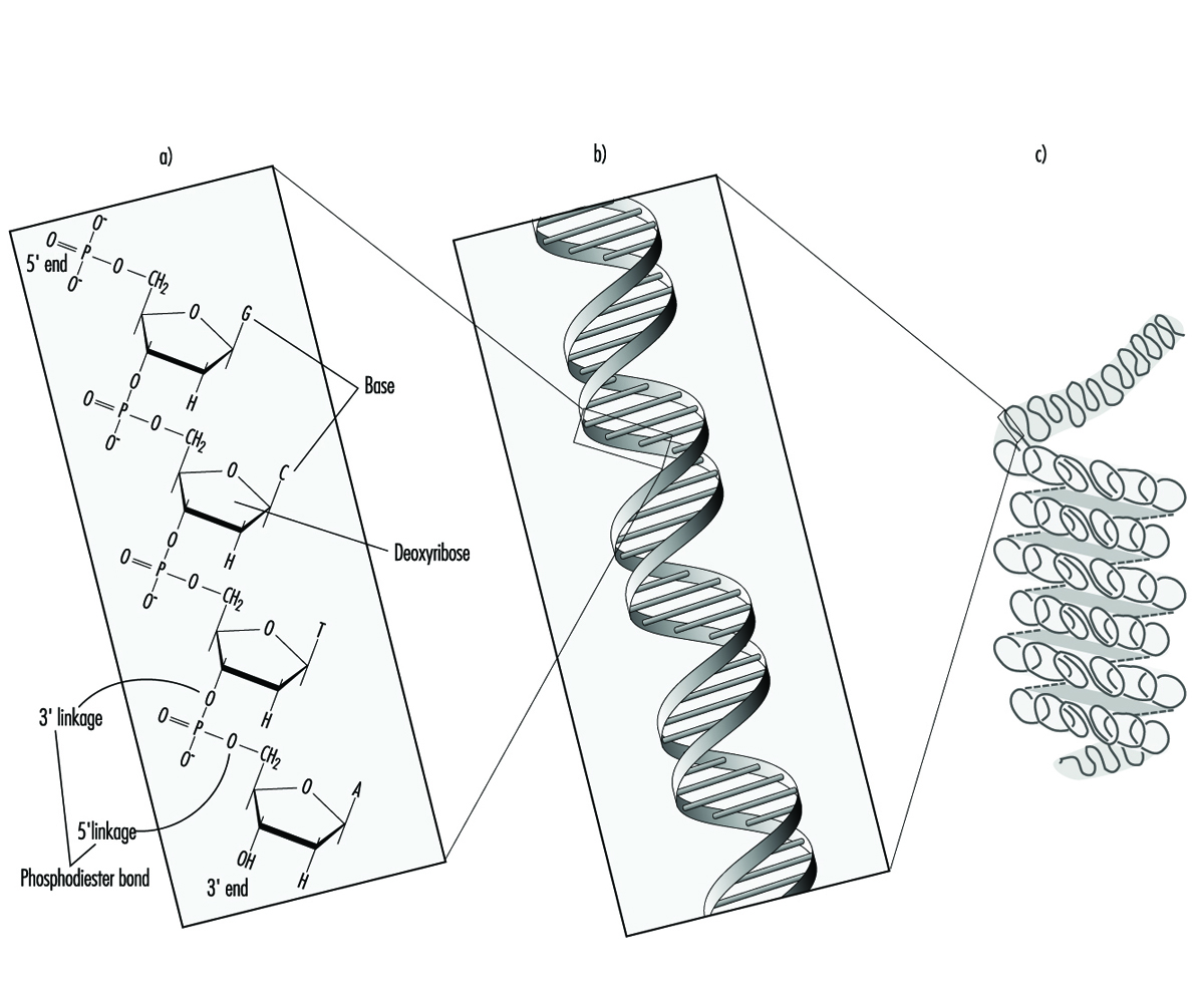 Using RNA and an array of different proteins, the cell ultimately deciphers the information encoded by the linear sequence of bases within specific regions of DNA (genes) and produces proteins that are essential for basic cell survival as well as normal growth and differentiation. In essence, the nucleotides function like a biological alphabet which is used to code for amino acids, the building blocks of proteins.
When incorrect nucleotides are inserted or nucleotides are lost, or when unnecessary nucleotides are added during DNA synthesis, the mistake is called a mutation. It has been estimated that less than one mutation occurs for every 109 nucleotides incorporated during the normal replication of cells. Although mutations are not necessarily harmful, alterations causing inactivation or overexpression of important genes can result in a variety of disorders, including cancer, hereditary disease, developmental abnormalities, infertility and embryonic or perinatal death. Very rarely, a mutation can lead to enhanced survival; such occurrences are the basis of natural selection.
Although some chemicals react directly with DNA, most require metabolic activation. In the latter case, electrophilic intermediates such as epoxides or carbonium ions are ultimately responsible for inducing lesions at a variety of nucleophilic sites within the genetic material (figure 2). In other instances, genotoxicity is mediated by by-products of compound interaction with intracellular lipids, proteins, or oxygen.
Figure 2. Bioactivation of: a) benzo(a)pyrene; and b) N-nitrosodimethylamine
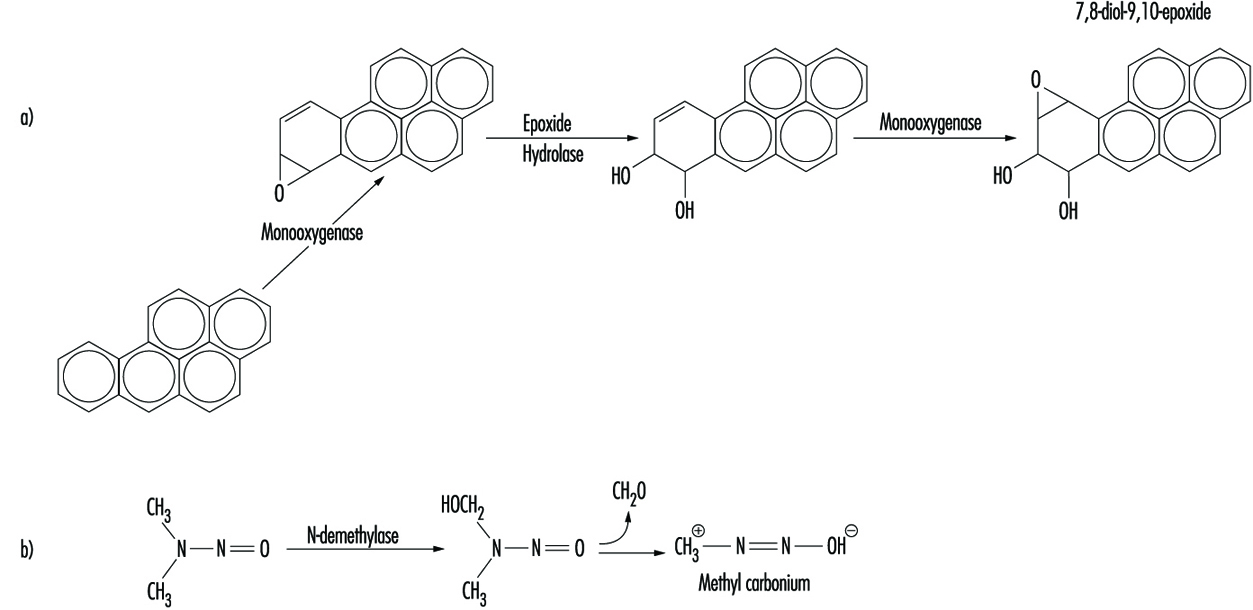
Because of their relative abundance in cells, proteins are the most frequent target of toxicant interaction. However, modification of DNA is of greater concern due to the central role of this molecule in regulating growth and differentiation through multiple generations of cells.
At the molecular level, electrophilic compounds tend to attack oxygen and nitrogen in DNA. The sites that are most prone to modification are illustrated in figure 3. Although oxygens within phosphate groups in the DNA backbone are also targets for chemical modification, damage to bases is thought to be biologically more relevant since these groups are considered to be the primary informational elements in the DNA molecule.
Figure 3. Primary sites of chemically-induced DNA damage
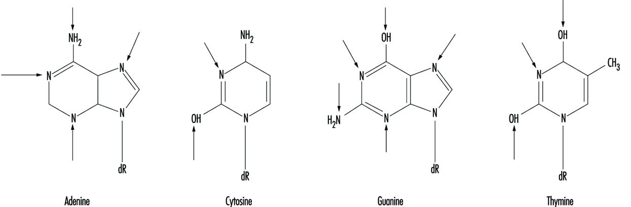
Compounds that contain one electrophilic moiety typically exert genotoxicity by producing mono-adducts in DNA. Similarly, compounds that contain two or more reactive moieties can react with two different nucleophilic centres and thereby produce intra- or inter-molecular crosslinks in genetic material (figure 4). Interstrand DNA-DNA and DNA-protein crosslinks can be particularly cytotoxic since they can form complete blocks to DNA replication. For obvious reasons, the death of a cell eliminates the possibility that it will be mutated or neoplastically transformed. Genotoxic agents can also act by inducing breaks in the phosphodiester backbone, or between bases and sugars (producing abasic sites) in DNA. Such breaks may be a direct result of chemical reactivity at the damage site, or may occur during the repair of one of the aforementioned types of DNA lesion.
Figure 4. Various types of damage to the protein-DNA complex

Over the past thirty to forty years, a variety of techniques have been developed to monitor the type of genetic damage induced by various chemicals. Such assays are described in detail elsewhere in this chapter and Encyclopaedia.
Misreplication of “microlesions” such as mono-adducts, abasic sites or single-strand breaks may ultimately result in nucleotide base-pair substitutions, or the insertion or deletion of short polynucleotide fragments in chromosomal DNA. In contrast, “macrolesions,” such as bulky adducts, crosslinks, or double-strand breaks may trigger the gain, loss or rearrangement of relatively large pieces of chromosomes. In any case, the consequences can be devastating to the organism since any one of these events can lead to cell death, loss of function or malignant transformation of cells. Exactly how DNA damage causes cancer is largely unknown. It is currently believed the process may involve inappropriate activation of proto-oncogenes such as myc and ras, and/or inactivation of recently identified tumour suppressor genes such as p53. Abnormal expression of either type of gene abrogates normal cellular mechanisms for controlling cell proliferation and/or differentiation.
The preponderance of experimental evidence indicates that the development of cancer following exposure to electrophilic compounds is a relatively rare event. This can be explained, in part, by the cell’s intrinsic ability to recognize and repair damaged DNA or the failure of cells with damaged DNA to survive. During repair, the damaged base, nucleotide or short stretch of nucleotides surrounding the damage site is removed and (using the opposite strand as a template) a new piece of DNA is synthesized and spliced into place. To be effective, DNA repair must occur with great accuracy prior to cell division, before opportunities for the propagation of mutation.
Clinical studies have shown that people with inherited defects in the ability to repair damaged DNA frequently develop cancer and/or developmental abnormalities at an early age (table 1). Such examples provide strong evidence linking accumulation of DNA damage to human disease. Similarly, agents that promote cell proliferation (such as tetradecanoylphorbol acetate) often enhance carcinogenesis. For these compounds, the increased likelihood of neoplastic transformation may be a direct consequence of a decrease in the time available for the cell to carry out adequate DNA repair.
Table 1. Hereditary, cancer-prone disorders that appear to involve defects in DNA repair
| Syndrome | Symptoms | Cellular phenotype |
| Ataxia telangiectasia | Neurological deterioration Immunodeficiency High incidence of lymphoma |
Hypersensitivity to ionizing radiation and certain alkylating agents. Dysregulated replication of damaged DNA (may indicate shortened time for DNA repair) |
| Bloom’s syndrome | Developmental abnormalities Lesions on exposed skin High incidence of tumours of the immune system and gastrointestinal tract |
High frequency of chromosomal aberrations Defective ligation of breaks associated with DNA repair |
| Fanconi’s anaemia | Growth retardation High incidence of leukaemia |
Hypersensitivity to crosslinking agents High frequency of chromosomal aberrations Defective repair of crosslinks in DNA |
| Hereditary nonpolyposis colon cancer | High incidence of colon cancer | Defect in DNA mismatch repair (when insertion of wrong nucleotide occurs during replication) |
| Xeroderma pigmentosum | High incidence of epithelioma on exposed areas of skin Neurological impairment (in many cases) |
Hypersensitivity to UV light and many chemical carcinogens Defects in excision repair and/or replication of damaged DNA |
The earliest theories on how chemicals interact with DNA can be traced back to studies conducted during the development of mustard gas for use in warfare. Further understanding grew out of efforts to identify anticancer agents that would selectively arrest the replication of rapidly dividing tumour cells. Increased public concern over hazards in our environment has prompted additional research into the mechanisms and consequences of chemical interaction with the genetic material. Examples of various types of chemicals which exert genotoxicity are presented in table 2.
Table 2. Examples of chemicals that exhibit genotoxicity in human cells
| Class of chemical | Example | Source of exposure | Probable genotoxic lesion |
| Aflatoxins | Aflatoxin B1 | Contaminated food | Bulky DNA adducts |
| Aromatic amines | 2-Acetylaminofluorene | Environmental | Bulky DNA adducts |
| Aziridine quinones | Mitomycin C | Cancer chemotherapy | Mono-adducts, interstrand crosslinks and single-strand breaks in DNA. |
| Chlorinated hydrocarbons | Vinyl chloride | Environmental | Mono-adducts in DNA |
| Metals and metal compounds | Cisplatin | Cancer chemotherapy | Both intra- and inter-strand crosslinks in DNA |
| Nickel compounds | Environmental | Mono-adducts and single-strand breaks in DNA | |
| Nitrogen mustards | Cyclophosphamide | Cancer chemotherapy | Mono-adducts and interstrand crosslinks in DNA |
| Nitrosamines | N-Nitrosodimethylamine | Contaminated food | Mono-adducts in DNA |
| Polycyclic aromatic hydrocarbons | Benzo(a)pyrene | Environmental | Bulky DNA adducts |
More...
Measuring Effects of Exposures
Epidemiology involves measuring the occurrence of disease and quantifying associations between diseases and exposures.
Measures of Disease Occurrence
Disease occurrence can be measured by frequencies (counts) but is better described by rates, which are composed of three elements: the number of people affected (numerator), the number of people in the source or base population (i.e., the population at risk) from which the affected persons come, and the time period covered. The denominator of the rate is the total person-time experienced by the source population. Rates allow more informative comparisons between populations of different sizes than counts alone. Risk, the probability of an individual developing disease within a specified time period, is a proportion, ranging from 0 to 1, and is not a rate per se. Attack rate, the proportion of people in a population who are affected within a specified time period, is technically a measure of risk, not a rate.
Disease-specific morbidity includes incidence, which refers to the number of persons who are newly diagnosed with the disease of interest. Prevalence refers to the number of existing cases. Mortality refers to the number of persons who die.
Incidence is defined as the number of newly diagnosed cases within a specified time period, whereas the incidence rate is this number divided by the total person-time experienced by the source population (table 1). For cancer, rates are usually expressed as annual rates per 100,000 people. Rates for other more common diseases may be expressed per a smaller number of people. For example, birth defect rates are usually expressed per 1,000 live births. Cumulative incidence, the proportion of people who become cases within a specified time period, is a measure of average risk for a population.
Table 1. Measures of disease occurrence: Hypothetical population observed for a five-year period
|
Newly diagnosed cases |
10 |
|
Previously diagnosed living cases |
12 |
|
Deaths, all causes* |
5 |
|
Deaths, disease of interest |
3 |
|
Persons in population |
100 |
|
Years observed |
5 |
|
Incidence |
10 persons |
|
Annual incidence rate |
|
|
Point prevalence (at end of year 5) |
(10 + 12 - 3) = 19 persons |
|
Period prevalence (five-year period) |
(10 + 12) = 22 persons |
|
Annual death rate |
|
|
Annual mortality rate |
|
*To simplify the calculations, this example assumes that all deaths occurred at the end of the five-year period so that all 100 persons in the population were alive for the full five years.
Prevalence includes point prevalence, the number of cases of disease at a point in time, and period prevalence, the total number of cases of a disease known to have existed at some time during a specified period.
Mortality, which concerns deaths rather than newly diagnosed cases of disease, reflects factors that cause disease as well as factors related to the quality of medical care, such as screening, access to medical care, and availability of effective treatments. Consequently, hypothesis-generating efforts and aetiological research may be more informative and easier to interpret when based on incidence rather than on mortality data. However, mortality data are often more readily available on large populations than incidence data.
The term death rate is generally accepted to mean the rate for deaths from all causes combined, whereas mortality rate is the rate of death from one specific cause. For a given disease, the case-fatality rate (technically a proportion, not a rate) is the number of persons dying from the disease during a specified time period divided by the number of persons with the disease. The complement of the case-fatality rate is the survival rate. The five-year survival rate is a common benchmark for chronic diseases such as cancer.
The occurrence of a disease may vary across subgroups of the population or over time. A disease measure for an entire population, without consideration of any subgroups, is called a crude rate. For example, an incidence rate for all age groups combined is a crude rate. The rates for the individual age groups are the age-specific rates. To compare two or more populations with different age distributions, age-adjusted (or, age-standardized) rates should be calculated for each population by multiplying each age-specific rate by the per cent of the standard population (e.g., one of the populations under study, the 1970 US population) in that age group, then summing over all age groups to produce an overall age-adjusted rate. Rates can be adjusted for factors other than age, such as race, gender or smoking status, if the category-specific rates are known.
Surveillance and evaluation of descriptive data can provide clues to disease aetiology, identify high-risk subgroups that may be suitable for intervention or screening programmes, and provide data on the effectiveness of such programmes. Sources of information that have been used for surveillance activities include death certificates, medical records, cancer registries, other disease registries (e.g., birth defects registries, end-stage renal disease registries), occupational exposure registries, health or disability insurance records and workmen’s compensation records.
Measures of Association
Epidemiology attempts to identify and quantify factors that influence disease. In the simplest approach, the occurrence of disease among persons exposed to a suspect factor is compared to the occurrence among persons unexposed. The magnitude of an association between exposure and disease can be expressed in either absolute or relative terms. (See also "Case Study: Measures").
Absolute effects are measured by rate differences and risk differences (table 2). A rate difference is one rate minus a second rate. For example, if the incidence rate of leukaemia among workers exposed to benzene is 72 per 100,000 person-years and the rate among non-exposed workers is 12 per 100,000 person-years, then the rate difference is 60 per 100,000 person-years. A risk difference is a difference in risks or cumulative incidence and can range from -1 to 1.
Table 2. Measures of association for a cohort study
|
Cases |
Person-years at risk |
Rate per 100,000 |
|
|
Exposed |
100 |
20,000 |
500 |
|
Unexposed |
200 |
80,000 |
250 |
|
Total |
300 |
100,000 |
300 |
Rate Difference (RD) = 500/100,000 - 250/100,000
= 250/100,000 per year
(146.06/100,000 - 353.94/100,000)*
Rate ratio (or relative risk) (RR) = ![]()
Attributable risk in the exposed (ARe) = 100/20,000 - 200/80,000
= 250/100,000 per year
Attributable risk per cent in the exposed (ARe%) =![]()
Population attributable risk (PAR) = 300/100,000 - 200/80,000
= 50/100,000 per year
Population attributable risk per cent (PAR%) =
![]()
* In parentheses 95% confidence intervals computed using the formulas in the boxes.
Relative effects are based on ratios of rates or risk measures, instead of differences. A rate ratio is the ratio of a rate in one population to the rate in another. The rate ratio has also been called the risk ratio, relative risk, relative rate, and incidence (or mortality) rate ratio. The measure is dimensionless and ranges from 0 to infinity. When the rate in two groups is similar (i.e., there is no effect from the exposure), the rate ratio is equal to unity (1). An exposure that increased risk would yield a rate ratio greater than unity, while a protective factor would yield a ratio between 0 and 1. The excess relative risk is the relative risk minus 1. For example, a relative risk of 1.4 may also be expressed as an excess relative risk of 40%.
In case-control studies (also called case-referent studies), persons with disease are identified (cases) and persons without disease are identified (controls or referents). Past exposures of the two groups are compared. The odds of being an exposed case is compared to the odds of being an exposed control. Complete counts of the source populations of exposed and unexposed persons are not available, so disease rates cannot be calculated. Instead, the exposed cases can be compared to the exposed controls by calculation of relative odds, or the odds ratio (table 3).
Table 3. Measures of association for case-control studies: Exposure to wood dust and adenocarcinoma of the nasal cavity and paranasal sinues
|
Cases |
Controls |
|
|
Exposed |
18 |
55 |
|
Unexposed |
5 |
140 |
|
Total |
23 |
195 |
Relative odds (odds ratio) (OR) = ![]()
Attributable risk per cent in the exposed (![]() ) =
) = ![]()
Population attributable risk per cent (PAR%) = ![]()
where ![]() = proportion of exposed controls = 55/195 = 0.28
= proportion of exposed controls = 55/195 = 0.28
* In parentheses 95% confidence intervals computed using the formulas in the box overleaf.
Source: Adapted from Hayes et al. 1986.
Relative measures of effect are used more frequently than absolute measures to report the strength of an association. Absolute measures, however, may provide a better indication of the public health impact of an association. A small relative increase in a common disease, such as heart disease, may affect more persons (large risk difference) and have more of an impact on public health than a large relative increase (but small absolute difference) in a rare disease, such as angiosarcoma of the liver.
Significance Testing
Testing for statistical significance is often performed on measures of effect to evaluate the likelihood that the effect observed differs from the null hypothesis (i.e., no effect). While many studies, particularly in other areas of biomedical research, may express significance by p-values, epidemiological studies typically present confidence intervals (CI) (also called confidence limits). A 95% confidence interval, for example, is a range of values for the effect measure that includes the estimated measure obtained from the study data and that which has 95% probability of including the true value. Values outside the interval are deemed to be unlikely to include the true measure of effect. If the CI for a rate ratio includes unity, then there is no statistically significant difference between the groups being compared.
Confidence intervals are more informative than p-values alone. A p-value’s size is determined by either or both of two reasons. Either the measure of association (e.g., rate ratio, risk difference) is large or the populations under study are large. For example, a small difference in disease rates observed in a large population may yield a highly significant p-value. The reasons for the large p-value cannot be identified from the p-value alone. Confidence intervals, however, allow us to disentangle the two factors. First, the magnitude of the effect is discernible by the values of the effect measure and the numbers encompassed by the interval. Larger risk ratios, for example, indicate a stronger effect. Second, the size of the population affects the width of the confidence interval. Small populations with statistically unstable estimates generate wider confidence intervals than larger populations.
The level of confidence chosen to express the variability of the results (the “statistical significance”) is arbitrary, but has traditionally been 95%, which corresponds to a p-value of 0.05. A 95% confidence interval has a 95% probability of containing the true measure of the effect. Other levels of confidence, such as 90%, are occasionally used.
Exposures can be dichotomous (e.g., exposed and unexposed), or may involve many levels of exposure. Effect measures (i.e., response) can vary by level of exposure. Evaluating exposure-response relationships is an important part of interpreting epidemiological data. The analogue to exposure-response in animal studies is “dose-response”. If the response increases with exposure level, an association is more likely to be causal than if no trend is observed. Statistical tests to evaluate exposure-response relationships include the Mantel extension test and the chi-square trend test.
Standardization
To take into account factors other than the primary exposure of interest and the disease, measures of association may be standardized through stratification or regression techniques. Stratification means dividing the populations into homogenous groups with respect to the factor (e.g., gender groups, age groups, smoking groups). Risk ratios or odds ratios are calculated for each stratum and overall weighted averages of the risk ratios or odds ratios are calculated. These overall values reflect the association between the primary exposure and disease, adjusted for the stratification factor, i.e., the association with the effects of the stratification factor removed.
A standardized rate ratio (SRR) is the ratio of two standardized rates. In other words, an SRR is a weighted average of stratum-specific rate ratios where the weights for each stratum are the person-time distribution of the non-exposed, or referent, group. SRRs for two or more groups may be compared if the same weights are used. Confidence intervals can be constructed for SRRs as for rate ratios.
The standardized mortality ratio (SMR) is a weighted average of age-specific rate ratios where the weights (e.g., person-time at risk) come from the group under study and the rates come from the referent population, the opposite of the situation in a SRR. The usual referent population is the general population, whose mortality rates may be readily available and based on large numbers and thus are more stable than using rates from a non-exposed cohort or subgroup of the occupational population under study. Using the weights from the cohort instead of the referent population is called indirect standardization. The SMR is the ratio of the observed number of deaths in the cohort to the expected number, based on the rates from the referent population (the ratio is typically multiplied by 100 for presentation). If no association exists, the SMR equals 100. It should be noted that because the rates come from the referent population and the weights come from the study group, two or more SMRs tend not to be comparable. This non-comparability is often forgotten in the interpretation of epidemiological data, and erroneous conclusions can be drawn.
Healthy Worker Effect
It is very common for occupational cohorts to have lower total mortality than the general population, even if the workers are at increased risk for selected causes of death from workplace exposures. This phenomenon, called the healthy worker effect, reflects the fact that any group of employed persons is likely to be healthier, on average, than the general population, which includes workers and persons unable to work due to illnesses and disabilities. The overall mortality rate in the general population tends to be higher than the rate in workers. The effect varies in strength by cause of death. For example, it appears to be less important for cancer in general than for chronic obstructive lung disease. One reason for this is that it is likely that most cancers would not have developed out of any predisposition towards cancer underlying job/career selection at a younger age. The healthy worker effect in a given group of workers tends to diminish over time.
Proportional Mortality
Sometimes a complete tabulation of a cohort (i.e., person-time at risk) is not available and there is information only on the deaths or some subset of deaths experienced by the cohort (e.g., deaths among retirees and active employees, but not among workers who left employment before becoming eligible for a pension). Computation of person-years requires special methods to deal with person-time assessment, including life-table methods. Without total person-time information on all cohort members, regardless of disease status, SMRs and SRRs cannot be calculated. Instead, proportional mortality ratios (PMRs) can be used. A PMR is the ratio of the observed number of deaths due to a specific cause in comparison to the expected number, based on the proportion of total deaths due to the specific cause in the referent population, multiplied by the number of total deaths in the study group, multiplied by 100.
Because the proportion of deaths from all causes combined must equal 1 (PMR=100), some PMRs may appear to be in excess, but are actually artificially inflated due to real deficits in other causes of death. Similarly, some apparent deficits may merely reflect real excesses of other causes of death. For example, if aerial pesticide applicators have a large real excess of deaths due to accidents, the mathematical requirement that the PMR for all causes combined equal 100 may cause some one or other causes of death to appear deficient even if the mortality is excessive. To ameliorate this potential problem, researchers interested primarily in cancer can calculate proportionate cancer mortality ratios (PCMRs). PCMRs compare the observed number of cancer deaths to the number expected based on the proportion of total cancer deaths (rather than all deaths) for the cancer of interest in the referent population multiplied by the total number of cancer deaths in the study group, multiplied by 100. Thus, the PCMR will not be affected by an aberration (excess or deficit) in a non-cancer cause of death, such as accidents, heart disease or non-malignant lung disease.
PMR studies can better be analysed using mortality odds ratios (MORs), in essence analysing the data as if they were from a case-control study. The “controls” are the deaths from a subset of all deaths that are thought to be unrelated to the exposure under study. For example, if the main interest of the study were cancer, mortality odds ratios could be calculated comparing exposure among the cancer deaths to exposure among the cardiovascular deaths. This approach, like the PCMR, avoids the problems with the PMR which arise when a fluctuation in one cause of death affects the apparent risk of another simply because the overall PMR must equal 100. The choice of the control causes of death is critical, however. As mentioned above, they must not be related to the exposure, but the possible relationship between exposure and disease may not be known for many potential control diseases.
Attributable Risk
There are measures available which express the amount of disease that would be attributable to an exposure if the observed association between the exposure and disease were causal. The attributable risk in the exposed (ARe) is the disease rate in the exposed minus the rate in the unexposed. Because disease rates cannot be measured directly in case-control studies, the ARe is calculable only for cohort studies. A related, more intuitive, measure, the attributable risk percent in the exposed (ARe%), can be obtained from either study design. The ARe% is the proportion of cases arising in the exposed population that is attributable to the exposure (see table 2 and table 3 for formula). The ARe% is the rate ratio (or the odds ratio) minus 1, divided by the rate ratio (or odds ratio), multiplied by 100.
The population attributable risk (PAR) and the population attributable risk per cent (PAR%), or aetiological fraction, express the amount of disease in the total population, which is comprised of exposed and unexposed persons, that is due to the exposure if the observed association is causal. The PAR can be obtained from cohort studies (table 28.3 ) and the PAR% can be calculated in both cohort and case-control studies (table 2 and table 3).
Representativeness
There are several measures of risk that have been described. Each assumes underlying methods for counting events and in the representatives of these events to a defined group. When results are compared across studies, an understanding of the methods used is essential for explaining any observed differences.
Biomechanics
Aims and Principles
Biomechanics is a discipline that approaches the study of the body as though it were solely a mechanical system: all parts of the body are likened to mechanical structures and are studied as such. The following analogies may, for example, be drawn:
- bones: levers, structural members
- flesh: volumes and masses
- joints: bearing surfaces and articulations
- joint linings: lubricants
- muscles: motors, springs
- nerves: feedback control mechanisms
- organs: power supplies
- tendons: ropes
- tissue: springs
- body cavities: balloons.
The main aim of biomechanics is to study the way the body produces force and generates movement. The discipline relies primarily on anatomy, mathematics and physics; related disciplines are anthropometry (the study of human body measurements), work physiology and kinesiology (the study of the principles of mechanics and anatomy in relation to human movement).
In considering the occupational health of the worker, biomechanics helps to understand why some tasks cause injury and ill health. Some relevant types of adverse health effect are muscle strain, joint problems, back problems and fatigue.
Back strains and sprains and more serious problems involving the intervertebral discs are common examples of workplace injuries that can be avoided. These often occur because of a sudden particular overload, but may also reflect the exertion of excessive forces by the body over many years: problems may occur suddenly or may take time to develop. An example of a problem that develops over time is “seamstress’s finger”. A recent description describes the hands of a woman who, after 28 years of work in a clothing factory, as well as sewing in her spare time, developed hardened thickened skin and an inability to flex her fingers (Poole 1993). (Specifically, she suffered from a flexion deformity of the right index finger, prominent Heberden’s nodes on the index finger and thumb of the right hand, and a prominent callosity on the right middle finger due to constant friction from the scissors.) X-ray films of her hands showed severe degenerative changes in the outermost joints of her right index and middle fingers, with loss of joint space, articular sclerosis (hardening of tissue), osteophytes (bony growths at the joint) and bone cysts.
Inspection at the workplace showed that these problems were due to repeated hyperextension (bending up) of the outermost finger joint. Mechanical overload and restriction in blood flow (visible as a whitening of the finger) would be maximal across these joints. These problems developed in response to repeated muscle exertion in a site other than the muscle.
Biomechanics helps to suggest ways of designing tasks to avoid these types of injuries or of improving poorly designed tasks. Remedies for these particular problems are to redesign the scissors and to alter the sewing tasks to remove the need for the actions performed.
Two important principles of biomechanics are:
- Muscles come in pairs. Muscles can only contract, so for any joint there must be one muscle (or muscle group) to move it one way and a corresponding muscle (or muscle group) to move it in the opposite direction. Figure 1 illustrates the point for the elbow joint.
- Muscles contract most efficiently when the muscle pair is in relaxed balance. The muscle acts most efficiently when it is in the midrange of the joint it flexes. This is so for two reasons: first, if the muscle tries to contract when it is shortened, it will pull against the elongated opposing muscle. Because the latter is stretched, it will apply an elastic counterforce that the contracting muscle must overcome. Figure 2 shows the way in which muscle force varies with muscle length.
Figure 1. Skeletal muscles occur in pairs in order to initiate or reverse a movement
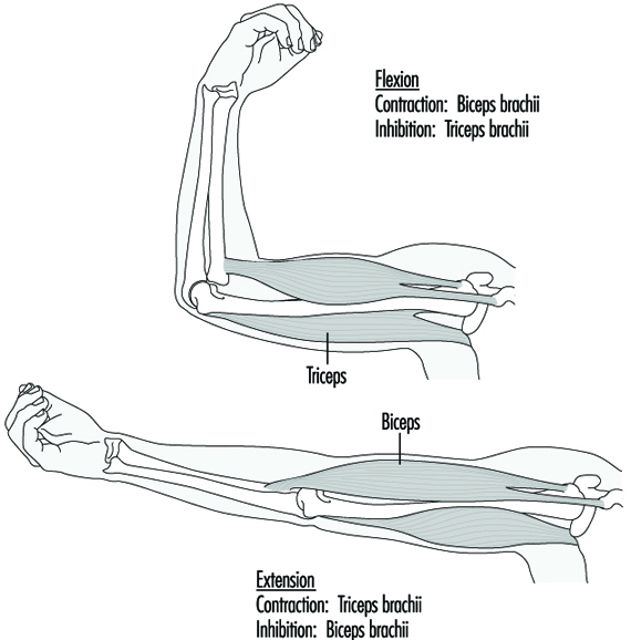
Figure 2. Muscle tension varies with muscle length

Second, if the muscle tries to contract at other than the midrange of the movement of the joint, it will operate at a mechanical disadvantage. Figure 3 illustrates the change in mechanical advantage for the elbow in three different positions.
Figure 3. Optimal positions for joint movement

An important criterion for work design follows from these principles: Work should be arranged so that it occurs with the opposing muscles of each joint in relaxed balance. For most joints, this means that the joint should be at about its midrange of movement.
This rule also means that muscle tension will be at a minimum while a task is performed. One example of the infringement of the rule is the overuse syndrome (RSI, or repetitive strain injury) which affects the muscles of the top of the forearm in keyboard operators who habitually operate with the wrist flexed up. Often this habit is forced on the operator by the design of the keyboard and workstation.
Applications
The following are some examples illustrating the application of biomechanics.
The optimum diameter of tool handles
The diameter of a handle affects the force that the muscles of the hand can apply to a tool. Research has shown that the optimum handle diameter depends on the use to which the tool is put. For exerting thrust along the line of the handle, the best diameter is one that allows the fingers and thumb to assume a slightly overlapping grip. This is about 40 mm. To exert torque, a diameter of about 50-65 mm is optimal. (Unfortunately, for both purposes most handles are smaller than these values.)
The use of pliers
As a special case of a handle, the ability to exert force with pliers depends on the handle separation, as shown in figure 4.
Figure 4. Grip strength of pliers jaws exerted by male and female users as a function of handle separation
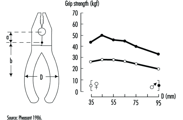
Seated posture
Electromyography is a technique that can be used to measure muscle tension. In a study of the tension in the erector spinae muscles (of the back) of seated subjects, it was found that leaning back (with the backrest inclined) reduced the tension in these muscles. The effect can be explained because the backrest takes more of the weight of the upper body.
X-ray studies of subjects in a variety of postures showed that the position of relaxed balance of the muscles that open and close the hip joint corresponds to a hip angle of about 135º. This is close to the position (128º) naturally adopted by this joint in weightless conditions (in space). In the seated posture, with an angle of 90º at the hip, the hamstring muscles that run over both the knee and hip joints tend to pull the sacrum (the part of the vertebral column that connects with the pelvis) into a vertical position. The effect is to remove the natural lordosis (curvature) of the lumbar spine; chairs should have appropriate backrests to correct for this effort.
Screwdriving
Why are screws inserted clockwise? The practice probably arose in unconscious recognition that the muscles that rotate the right arm clockwise (most people are right-handed) are larger (and therefore more powerful) that the muscles that rotate it anticlockwise.
Note that left-handed people will be at a disadvantage when inserting screws by hand. About 9% of the population are left-handed and will therefore require special tools in some situations: scissors and can openers are two such examples.
A study of people using screwdrivers in an assembly task revealed a more subtle relation between a particular movement and a particular health problem. It was found that the greater the elbow angle (the straighter the arm), the more people had inflammation at the elbow. The reason for this effect is that the muscle that rotates the forearm (the biceps) also pulls the head of the radius (lower arm bone) onto the capitulum (rounded head) of the humerus (upper arm bone). The increased force at the higher elbow angle caused greater frictional force at the elbow, with consequent heating of the joint, leading to the inflammation. At the higher angle, the muscle also had to pull with greater force to effect the screwing action, so a greater force was applied than would have been required with the elbow at about 90º. The solution was to move the task closer to the operators to reduce the elbow angle to about 90º.
The cases above demonstrate that a proper understanding of anatomy is required for the application of biomechanics in the workplace. Designers of tasks may need to consult experts in functional anatomy to anticipate the types of problems discussed. (The Pocket Ergonomist (Brown and Mitchell 1986) based on electromyographical research, suggests many ways of reducing physical discomfort at work.)
Manual Material Handling
The term manual handling includes lifting, lowering, pushing, pulling, carrying, moving, holding and restraining, and encompasses a large part of the activities of working life.
Biomechanics has obvious direct relevance to manual handling work, since muscles must move to carry out tasks. The question is: how much physical work can people be reasonably expected to do? The answer depends on the circumstances; there are really three questions that need to be asked. Each one has an answer that is based on scientifically researched criteria:
- How much can be handled without damage to the body (in the form, for example, of muscle strain, disc injury or joint problems)? This is called the biomechanical criterion.
- How much can be handled without overexerting the lungs (breathing hard to the point of panting)? This is called the physiological criterion.
- How much do people feel able to handle comfortably? This is called the psychophysical criterion.
There is a need for these three different criteria because there are three broadly different reactions that can occur to lifting tasks: if the work goes on all day, the concern will be how the person feels about the task—the psychophysical criterion; if the force to be applied is large, the concern would be that muscles and joints are not overloaded to the point of damage—the biomechanical criterion; and if the rate of work is too great, then it may well exceed the physiological criterion, or the aerobic capacity of the person.
Many factors determine the extent of the load placed on the body by a manual handling task. All of them suggest opportunities for control.
Posture and Movements
If the task requires a person to twist or reach forward with a load, the risk of injury is greater. The workstation can often be redesigned to prevent these actions. More back injuries occur when the lift begins at ground level compared to mid-thigh level, and this suggests simple control measures. (This applies to high lifting as well.)
The load.
The load itself may influence handling because of its weight and its location. Other factors, such as its shape, its stability, its size and its slipperiness may all affect the ease of a handling task.
Organization and environment.
The way work is organized, both physically and over time (temporally), also influences handling. It is better to spread the burden of unloading a truck in a delivery bay over several people for an hour rather than to ask one worker to spend all day on the task. The environment influences handling—poor light, cluttered or uneven floors and poor housekeeping may all cause a person to stumble.
Personal factors.
Personal handling skills, the age of the person and the clothing worn also can influence handling requirements. Education for training and lifting are required both to provide necessary information and to allow time for the development of the physical skills of handling. Younger people are more at risk; on the other hand, older people have less strength and less physiological capacity. Tight clothing can increase the muscle force required in a task as people strain against the tight cloth; classic examples are the nurse’s smock uniform and tight overalls when people do work above their heads.
Recommended Weight Limits
The points mentioned above indicate that it is impossible to state a weight that will be “safe” in all circumstances. (Weight limits have tended to vary from country to country in an arbitrary manner. Indian dockers, for example, were once “allowed” to lift 110 kg, while their counterparts in the former People’s Democratic Republic of Germany were “limited” to 32 kg.) Weight limits have also tended to be too great. The 55 kg suggested in many countries is now thought to be far too great on the basis of recent scientific evidence. The National Institute for Occupational Safety and Health (NIOSH) in the United States has adopted 23 kg as a load limit in 1991 (Waters et al. 1993).
Each lifting task needs to be assessed on its own merits. A useful approach to determining a weight limit for a lifting task is the equation developed by NIOSH:
RWL = LC x HM x VM x DM x AM x CM x FM
Where
RWL = recommended weight limit for the task in question
HM = the horizontal distance from the centre of gravity of the load to the midpoint between the ankles (minimum 15 cm, maximum 80 cm)
VM = the vertical distance between the centre of gravity of the load and the floor at the start of the lift (maximum 175 cm)
DM = the vertical travel of the lift (minimum 25 cm, maximum 200 cm)
AM = asymmetry factor–the angle the task deviates from straight out in front of the body
CM = coupling multiplier–the ability to get a good grip on the item to be lifted, which is found in a reference table
FM = frequency multipliers–the frequency of the lifting.
All variables of length in the equation are expressed in units of centimetres. It should be noted that 23 kg is the maximum weight that NIOSH recommends for lifting. This has been reduced from 40 kg after observation of many people doing many lifting tasks has revealed that the average distance from the body of the start of the lift is 25 cm, not the 15 cm assumed in an earlier version of the equation (NIOSH 1981).
Lifting index.
By comparing the weight to be lifted in the task and the RWL, a lifting index (LI) can be obtained according to the relationship:
LI=(weight to be handled)/RWL.
Therefore, particularly valuable use of the NIOSH equation is the placing of lifting tasks in order of severity, using the lifting index to set priorities for action. (The equation has a number of limitations, however, that need to be understood for its most effective application. See Waters et al. 1993).
Estimating Spinal Compression Imposed by the Task
Computer software is available to estimate the spinal compression produced by a manual handling task. The 2D and 3D Static Strength Prediction Programs from the University of Michigan (“Backsoft”) estimate spinal compression. The inputs required to the program are:
- the posture in which the handling activity is performed
- the force exerted
- the direction of the force exertion
- the number of hands exerting the force
- the percentile of the population under study.
The 2D and 3D programs differ in that the 3D software allows computations applying to postures in three dimensions. The program output gives spinal compression data and lists the percentage of the population selected that would be able to do the particular task without exceeding suggested limits for six joints: ankle, knee, hip, first lumbar disc-sacrum, shoulder, and elbow. This method also has a number of limitations that need to be fully understood in order to derive maximum value out of the program.
Immunotoxicology
The functions of the immune system are to protect the body from invading infectious agents and to provide immune surveillance against arising tumour cells. It has a first line of defence that is non-specific and that can initiate effector reactions itself, and an acquired specific branch, in which lymphocytes and antibodies carry the specificity of recognition and subsequent reactivity towards the antigen.
Immunotoxicology has been defined as “the discipline concerned with the study of the events that can lead to undesired effects as a result of interaction of xenobiotics with the immune system. These undesired events may result as a consequence of (1) a direct and/or indirect effect of the xenobiotic (and/or its biotransformation product) on the immune system, or (2) an immunologically based host response to the compound and/or its metabolite(s), or host antigens modified by the compound or its metabolites” (Berlin et al. 1987).
When the immune system acts as a passive target of chemical insults, the result can be decreased resistance to infection and certain forms of neoplasia, or immune disregulation/stimulation that can exacerbate allergy or auto-immunity. In the case that the immune system responds to the antigenic specificity of the xenobiotic or host antigen modified by the compound, toxicity can become manifest as allergies or autoimmune diseases.
Animal models to investigate chemical-induced immune suppression have been developed, and a number of these methods are validated (Burleson, Munson, and Dean 1995; IPCS 1996). For testing purposes, a tiered approach is followed to make an adequate selection from the overwhelming number of assays available. Generally, the objective of the first tier is to identify potential immunotoxicants. If potential immunotoxicity is identified, a second tier of testing is performed to confirm and characterize further the changes observed. Third-tier investigations include special studies on the mechanism of action of the compound. Several xenobiotics have been identified as immunotoxicants causing immunosuppression in such studies with laboratory animals.
The database on immune function disturbances in humans by environmental chemicals is limited (Descotes 1986; NRC Subcommittee on Immunotoxicology 1992). The use of markers of immunotoxicity has received little attention in clinical and epidemiological studies to investigate the effect of these chemicals on human health. Such studies have not been performed frequently, and their interpretation often does not permit unequivocal conclusions to be drawn, due for instance to the uncontrolled nature of exposure. Therefore, at present, immunotoxicity assessment in rodents, with subsequent extrapolation to man, forms the basis of decisions regarding hazard and risk.
Hypersensitivity reactions, notably allergic asthma and contact dermatitis, are important occupational health problems in industrialized countries (Vos, Younes and Smith 1995). The phenomenon of contact sensitization was investigated first in the guinea pig (Andersen and Maibach 1985). Until recently this has been the species of choice for predictive testing. Many guinea pig test methods are available, the most frequently employed being the guinea pig maximization test and the occluded patch test of Buehler. Guinea pig tests and newer approaches developed in mice, such as ear swelling tests and the local lymph node assay, provide the toxicologist with the tools to assess skin sensitization hazard. The situation with respect to sensitization of the respiratory tract is very different. There are, as yet, no well-validated or widely accepted methods available for the identification of chemical respiratory allergens although progress in the development of animal models for the investigation of chemical respiratory allergy has been achieved in the guinea pig and mouse.
Human data show that chemical agents, in particular drugs, can cause autoimmune diseases (Kammüller, Bloksma and Seinen 1989). There are a number of experimental animal models of human autoimmune diseases. Such comprise both spontaneous pathology (for example systemic lupus erythematosus in New Zealand Black mice) and autoimmune phenomena induced by experimental immunization with a cross-reactive autoantigen (for example the H37Ra adjuvant induced arthritis in Lewis strain rats). These models are applied in the preclinical evaluation of immunosuppressive drugs. Very few studies have addressed the potential of these models for assessment of whether a xenobiotic exacerbates induced or congenital autoimmunity. Animal models that are suitable to investigate the ability of chemicals to induce autoimmune diseases are virtually lacking. One model that is used to a limited extent is the popliteal lymph node assay in mice. Like the situation in humans, genetic factors play a crucial role in the development of autoimmune disease (AD) in laboratory animals, which will limit the predictive value of such tests.
The Immune System
The major function of the immune system is defence against bacteria, viruses, parasites, fungi and neoplastic cells. This is achieved by the actions of various cell types and their soluble mediators in a finely tuned concert. The host defence can be roughly divided into non-specific or innate resistance and specific or acquired immunity mediated by lymphocytes (Roitt, Brostoff and Male 1989).
Components of the immune system are present throughout the body (Jones et al. 1990). The lymphocyte compartment is found within lymphoid organs (figure 1). The bone marrow and thymus are classified as primary or central lymphoid organs; the secondary or peripheral lymphoid organs include lymph nodes, spleen and lymphoid tissue along secretory surfaces such as the gastrointestinal and respiratory tracts, the so-called mucosa-associated lymphoid tissue (MALT). About half of the body’s lymphocytes are located at any one time in MALT. In addition the skin is an important organ for the induction of immune responses to antigens present on the skin. Important in this process are epidermal Langerhans cells that have an antigen-presenting function.
Figure 1. Primary and secondary lymphoid organs and tissues
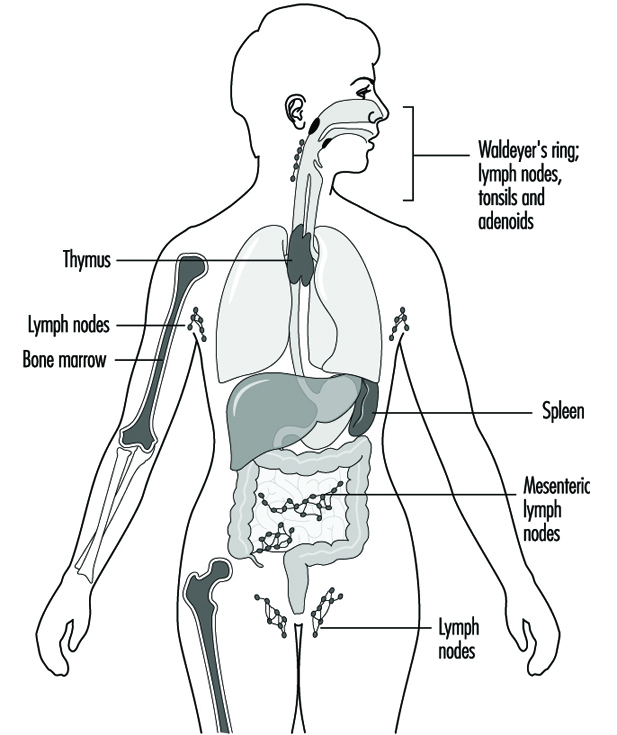
Phagocytic cells of the monocyte/macrophage lineage, called the mononuclear phagocyte system (MPS), occur in lymphoid organs and also at extranodal sites; the extranodal phagocytes include Kupffer cells in the liver, alveolar macrophages in the lung, mesangial macrophages in the kidney and glial cells in the brain. Polymorphonuclear leukocytes (PMNs) are present mainly in blood and bone marrow, but accumulate at sites of inflammation.
Non-specific defence
A first line of defence to micro-organisms is executed by a physical and chemical barrier, such as at the skin, the respiratory tract and the alimentary tract. This barrier is helped by non-specific protective mechanisms including phagocytic cells, such as macrophages and polymorphonuclear leukocytes, which are able to kill pathogens, and natural killer cells, which can lyse tumour cells and virus-infected cells. The complement system and certain microbial inhibitors (e.g., lysozyme) also take part in the non-specific response.
Specific immunity
After initial contact of the host with the pathogen, specific immune responses are induced. The hallmark of this second line of defence is specific recognition of determinants, so-called antigens or epitopes, of the pathogens by receptors on the cell surface of B- and T-lymphocytes. Following interaction with the specific antigen, the receptor-bearing cell is stimulated to undergo proliferation and differentiation, producing a clone of progeny cells that are specific for the eliciting antigen. The specific immune responses help the non-specific defence presented to the pathogens by stimulating the efficacy of the non-specific responses. A fundamental characteristic of specific immunity is that memory develops. Secondary contact with the same antigen provokes a faster and more vigorous but well-regulated response.
The genome does not have the capacity to carry the codes of an array of antigen receptors sufficient to recognize the number of antigens that can be encountered. The repertoire of specificity develops by a process of gene rearrangements. This is a random process, during which various specificities are brought about. This includes specificities for self components, which are undesirable. A selection process that takes place in the thymus (T cells), or bone marrow (B cells) operates to delete these undesirable specificities.
Normal immune effector function and homeostatic regulation of the immune response is dependent upon a variety of soluble products, known collectively as cytokines, which are synthesized and secreted by lymphocytes and by other cell types. Cytokines have pleiotropic effects on immune and inflammatory responses. Cooperation between different cell populations is required for the immune response—the regulation of antibody responses, the accumulation of immune cells and molecules at inflammatory sites, the initiation of acute phase responses, the control of macrophage cytotoxic function and many other processes central to host resistance. These are influenced by, and in many cases are dependent upon, cytokines acting individually or in concert.
Two arms of specific immunity are recognized—humoral immunity and cell-mediated or cellular immunity:
Humoral immunity. In the humoral arm B-lymphocytes are stimulated following recognition of antigen by cell-surface receptors. Antigen receptors on B-lymphocytes are immunoglobulins (Ig). Mature B cells (plasma cells) start the production of antigen-specific immunoglobulins that act as antibodies in serum or along mucosal surfaces. There are five major classes of immunoglobulins: (1) IgM, pentameric Ig with optimal agglutinating capacity, which is first produced after antigenic stimulation; (2) IgG, the main Ig in circulation, which can pass the placenta; (3) IgA, secretory Ig for the protection of mucosal surfaces; (4) IgE, Ig fixing to mast cells or basophilic granulocytes involved in immediate hypersensitivity reactions and (5) IgD, whose major function is as a receptor on B-lymphocytes.
Cell-mediated immunity. The cellular arm of the specific immune system is mediated by T-lymphocytes. These cells also have antigen receptors on their membranes. They recognize antigen if presented by antigen presenting cells in the context of histocompatibility antigens. Hence, these cells have a restriction in addition to the antigen specificity. T cells function as helper cells for various (including humoral) immune responses, mediate recruitment of inflammatory cells, and can, as cytotoxic T cells, kill target cells after antigen-specific recognition.
Mechanisms of Immunotoxicity
Immunosuppression
Effective host resistance is dependent upon the functional integrity of the immune system, which in turn requires that the component cells and molecules which orchestrate immune responses are available in sufficient numbers and in an operational form. Congenital immunodeficiencies in humans are often characterized by defects in certain stem cell lines, resulting in impaired or absent production of immune cells. By analogy with congenital and acquired human immunodeficiency diseases, chemical-induced immunosuppression may result simply from a reduced number of functional cells (IPCS 1996). The absence, or reduced numbers, of lymphocytes may have more or less profound effects on immune status. Some immunodeficiency states and severe immunosuppression, as can occur in transplantation or cytostatic therapy, have been associated in particular with increased incidences of opportunistic infections and of certain neoplastic diseases. The infections can be bacterial, viral, fungal or protozoan, and the predominant type of infection depends on the associated immunodeficiency. Exposure to immunosuppressive environmental chemicals may be expected to result in more subtle forms of immunosuppression, which may be difficult to detect. These may lead, for example, to an increased incidence of infections such as influenza or the common cold.
In view of the complexity of the immune system, with the wide variety of cells, mediators and functions that form a complicated and interactive network, immunotoxic compounds have numerous opportunities to exert an effect. Although the nature of the initial lesions induced by many immunotoxic chemicals have not yet been elucidated, there is increasing information available, mostly derived from studies in laboratory animals, regarding the immunobiological changes which result in depression of immune function (Dean et al. 1994). Toxic effects might occur at the following critical functions (and some examples are given of immunotoxic compounds affecting these functions):
- development and expansion of different stem cell populations (benzene exerts immunotoxic effects at the stem cell level, causing lymphocytopenia)
- proliferation of various lymphoid and myeloid cells as well as supportive tissues in which these cells mature and function (immunotoxic organotin compounds suppress the proliferative activity of lymphocytes in the thymic cortex through direct cytotoxicity; the thymotoxic action of 2,3,7,8-tetrachloro-dibenzo-p-dioxin (TCDD) and related compounds is likely due to an impaired function of thymic epithelial cells, rather than to direct toxicity for thymocytes)
- antigen uptake, processing and presentation by macrophages and other antigen-presenting cells (one of the targets of 7,12-dimethylbenz(a)anthracene (DMBA) and of lead is antigen presentation by macrophages; a target of ultraviolet radiation is the antigen-presenting Langerhans cell)
- regulatory function of T-helper and T-suppressor cells (T-helper cell function is impaired by organotins, aldicarb, polychlorinated biphenyls (PCBs), TCDD and DMBA; T-suppressor cell function is reduced by low-dose cyclophosphamide treatment)
- production of various cytokines or interleukins (benzo(a)pyrene (BP) suppresses interleukin-1 production; ultraviolet radiation alters production of cytokines by keratinocytes)
- synthesis of various classes of immunoglobulins IgM and IgG is suppressed following PCB and tributyltin oxide (TBT) treatment, and increased after hexachlorobenzene (HCB) exposure).
- complement regulation and activation (affected by TCDD)
- cytotoxic T cell function (3-methylcholanthrene (3-MC), DMBA, and TCDD suppress cytotoxic T cell activity)
- natural killer (NK) cell function (pulmonary NK activity is suppressed by ozone; splenic NK activity is impaired by nickel)
- macrophage and polymorphonuclear leukocyte chemotaxis and cytotoxic functions (ozone and nitrogen dioxide impair the phagocytic activity of alveolar macrophages).
Allergy
Allergy may be defined as the adverse health effects which result from the induction and elicitation of specific immune responses. When hypersensitivity reactions occur without involvement of the immune system the term pseudo-allergy is used. In the context of immunotoxicology, allergy results from a specific immune response to chemicals and drugs that are of interest. The ability of a chemical to sensitize individuals is generally related to its ability to bind covalently to body proteins. Allergic reactions may take a variety of forms and these differ with respect to both the underlying immunological mechanisms and the speed of the reaction. Four major types of allergic reactions have been recognized: Type I hypersensitivity reactions, which are effectuated by IgE antibody and where symptoms are manifest within minutes of exposure of the sensitized individual. Type II hypersensitivity reactions result from the damage or destruction of host cells by antibody. In this case symptoms become apparent within hours. Type III hypersensitivity, or Arthus, reactions are also antibody mediated, but against soluble antigen, and result from the local or systemic action of immune complexes. Type IV, or delayed-type hypersensitivity, reactions are effected by T-lymphocytes and normally symptoms develop 24to 48hours following exposure of the sensitized individual.
The two types of chemical allergy of greatest relevance to occupational health are contact sensitivity or skin allergy and allergy of the respiratory tract.
Contact hypersensitivity. A large number of chemicals are able to cause skin sensitization. Following topical exposure of a susceptible individual to a chemical allergen, a T-lymphocyte response is induced in the draining lymph nodes. In the skin the allergen interacts directly or indirectly with epidermal Langerhans cells, which transport the chemical to the lymph nodes and present it in an immunogenic form to responsive T-lymphocytes. Allergen- activated T-lymphocytes proliferate, resulting in clonal expansion. The individual is now sensitized and will respond to a second dermal exposure to the same chemical with a more aggressive immune response, resulting in allergic contact dermatitis. The cutaneous inflammatory reaction which characterizes allergic contact dermatitis is secondary to the recognition of the allergen in the skin by specific T-lymphocytes. These lymphocytes become activated, release cytokines and cause the local accumulation of other mononuclear leukocytes. Symptoms develop some 24 to 48 hours following exposure of the sensitized individual, and allergic contact dermatitis therefore represents a form of delayed-type hypersensitivity. Common causes of allergic contact dermatitis include organic chemicals (such as 2,4-dinitrochlorobenzene), metals (such as nickel and chromium) and plant products (such as urushiol from poison ivy).
Respiratory hypersensitivity. Respiratory hypersensitivity is usually considered to be a Type I hypersensitivity reaction. However, late phase reactions and the more chronic symptoms associated with asthma may involve cell-mediated (Type IV) immune processes. The acute symptoms associated with respiratory allergy are effected by IgE antibody, the production of which is provoked following exposure of the susceptible individual to the inducing chemical allergen. The IgE antibody distributes systemically and binds, via membrane receptors, to mast cells which are found in vascularized tissues, including the respiratory tract. Following inhalation of the same chemical a respiratory hypersensitivity reaction will be elicited. Allergen associates with protein and binds to, and cross-links, IgE antibody bound to mast cells. This in turn causes the degranulation of mast cells and the release of inflammatory mediators such as histamine and leukotrienes. Such mediators cause bronchoconstriction and vasodilation, resulting in the symptoms of respiratory allergy; asthma and/or rhinitis. Chemicals known to cause respiratory hypersensitivity in man include acid anhydrides (such as trimellitic anhydride), some diisocyanates (such as toluene diisocyanate), platinum salts and some reactive dyes. Also, chronic exposure to beryllium is known to cause hypersensitivity lung disease.
Autoimmunity
Autoimmunity can be defined as the stimulation of specific immune responses directed against endogenous “self” antigens. Induced autoimmunity can result either from alterations in the balance of regulatory T-lymphocytes or from the association of a xenobiotic with normal tissue components such as to render them immunogenic (“altered self”). Drugs and chemicals known to incidentally induce or exacerbate effects like those of autoimmune disease (AD) in susceptible individuals are low molecular weight compounds (molecular weight 100 to 500) that are generally considered to be not immunogenic themselves. The mechanism of AD by chemical exposure is mostly unknown. Disease can be produced directly by means of circulating antibody, indirectly through the formation of immune complexes, or as a consequence of cell-mediated immunity, but likely occurs through a combination of mechanisms. The pathogenesis is best known in immune haemolytic disorders induced by drugs:
- The drug can attach to the red-cell membrane and interact with a drug-specific antibody.
- The drug can alter the red-cell membrane so that the immune system regards the cell as foreign.
- The drug and its specific antibody form immune complexes that adhere to the red-cell membrane to produce injury.
- Red-cell sensitization occurs due to the production of red-cell autoantibody.
A variety of chemicals and drugs, in particular the latter, have been found to induce autoimmune-like responses (Kamüller, Bloksma and Seinen 1989). Occupational exposure to chemicals may incidentally lead to AD-like syndromes. Exposure to monomeric vinyl chloride, trichloroethylene, perchloroethylene, epoxy resins and silica dust may induce scleroderma-like syndromes. A syndrome similar to systemic lupus erythematosus (SLE) has been described after exposure to hydrazine. Exposure to toluene diisocyanate has been associated with the induction of thrombocytopenic purpura. Heavy metals such as mercury have been implicated in some cases of immune complex glomerulonephritis.
Human Risk Assessment
The assessment of human immune status is performed mainly using peripheral blood for analysis of humoral substances like immunoglobulins and complement, and of blood leukocytes for subset composition and functionality of subpopulations. These methods are usually the same as those used to investigate humoral and cell-mediated immunity as well as nonspecific resistance of patients with suspected congenital immunodeficiency disease. For epidemiological studies (e.g., of occupationally exposed populations) parameters should be selected on the basis of their predictive value in human populations, validated animal models, and the underlying biology of the markers (see table 1). The strategy in screening for immunotoxic effects after (accidental) exposure to environmental pollutants or other toxicants is much dependent on circumstances, such as type of immunodeficiency to be expected, time between exposure and immune status assessment, degree of exposure and number of exposed individuals. The process of assessing the immunotoxic risk of a particular xenobiotic in humans is extremely difficult and often impossible, due largely to the presence of various confounding factors of endogenous or exogenous origin that influence the response of individuals to toxic damage. This is particularly true for studies which investigate the role of chemical exposure in autoimmune diseases, where genetic factors play a crucial role.
Table 1. Classification of tests for immune markers
| Test category | Characteristics | Specific tests |
| Basic-general Should be included with general panels |
Indicators of general health and organ system status | Blood urea nitrogen, blood glucose, etc. |
| Basic-immune Should be included with general panels |
General indicators of immune status Relatively low cost Assay methods are standardized among laboratories Results outside reference ranges are clinically interpretable |
Complete blood counts Serum IgG, IgA, IgM levels Surface marker phenotypes for major lymphocyte subsets |
| Focused/reflex Should be included when indicated by clinical findings, suspected exposures, or prior test results |
Indicators of specific immune functions/events Cost varies Assay methods are standardized among laboratories Results outside reference ranges are clinically interpretable |
Histocompatibility genotype Antibodies to infectious agents Total serum IgE Allergen-specific IgE Autoantibodies Skin tests for hypersensitivity Granulocyte oxidative burst Histopathology (tissue biopsy) |
| Research Should be included only with control populations and careful study design |
Indicators of general or specific immune functions/events Cost varies; often expensive Assay methods are usually not standardized among laboratories Results outside reference ranges are often not clinically interpretable |
In vitro stimulation assays Cell activation surface markers Cytokine serum concentrations Clonality assays (antibody, cellular, genetic) Cytotoxicity tests |
As adequate human data are seldom available, the assessment of risk for chemical-induced immunosuppression in humans is in the majority of cases based upon animal studies. The identification of potential immunotoxic xenobiotics is undertaken primarily in controlled studies in rodents. In vivo exposure studies present, in this regard, the optimal approach to estimate the immunotoxic potential of a compound. This is due to the multifactoral and complex nature of the immune system and of immune responses. In vitro studies are of increasing value in the elucidation of mechanisms of immunotoxicity. In addition, by investigating the effects of the compound using cells of animal and human origin, data can be generated for species comparison, which can be used in the “parallelogram” approach to improve the risk assessment process. If data are available for three cornerstones of the parallelogram (in vivo animal, and in vitro animal and human) it may be easier to predict the outcome at the remaining cornerstone, that is, the risk in humans.
When assessment of risk for chemical-induced immunosuppression has to rely solely upon data from animal studies, an approach can be followed in the extrapolation to man by the application of uncertainty factors to the no observed adverse effect level (NOAEL). This level can be based on parameters determined in relevant models, such as host resistance assays and in vivo assessment of hypersensitivity reactions and antibody production. Ideally, the relevance of this approach to risk assessment requires confirmation by studies in humans. Such studies should combine the identification and measurement of the toxicant, epidemiological data and immune status assessments.
To predict contact hypersensitivity, guinea pig models are available and have been used in risk assessment since the 1970s. Although sensitive and reproducible, these tests have limitations as they depend on subjective evaluation; this can be overcome by newer and more quantitative methods developed in the mouse. Regarding chemical-induced hypersensitivity induced by inhalation or ingestion of allergens, tests should be developed and evaluated in terms of their predictive value in man. When it comes to setting safe occupational exposure levels of potential allergens, consideration has to be given to the biphasic nature of allergy: the sensitization phase and the elicitation phase. The concentration required to elicit an allergic reaction in a previously sensitized individual is considerably lower than the concentration necessary to induce sensitization in the immunologically naïve but susceptible individual.
As animal models to predict chemical-induced autoimmunity are virtually lacking, emphasis should be given to the development of such models. For the development of such models, our knowledge of chemical-induced autoimmunity in humans should be advanced, including the study of genetic and immune system markers to identify susceptible individuals. Humans that are exposed to drugs that induce autoimmunity offer such an opportunity.
Options in Study Design
The epidemiologist is interested in relationships between variables, chiefly exposure and outcome variables. Typically, epidemiologists want to ascertain whether the occurrence of disease is related to the presence of a particular agent (exposure) in the population. The ways in which these relationships are studied may vary considerably. One can identify all persons who are exposed to that agent and follow them up to measure the incidence of disease, comparing such incidence with disease occurrence in a suitable unexposed population. Alternatively, one can simply sample from among the exposed and unexposed, without having a complete enumeration of them. Or, as a third alternative, one can identify all people who develop a disease of interest in a defined time period (“cases”) and a suitable group of disease-free individuals (a sample of the source population of cases), and ascertain whether the patterns of exposure differ between the two groups. Follow-up of study participants is one option (in so-called longitudinal studies): in this situation, a time lag exists between the occurrence of exposure and disease onset. One alternative option is a cross-section of the population, where both exposure and disease are measured at the same point in time.
In this article, attention is given to the common study designs—cohort, case-referent (case-control) and cross-sectional. To set the stage for this discussion, consider a large viscose rayon factory in a small town. An investigation into whether carbon disulphide exposure increases the risk of cardiovascular disease is started. The investigation has several design choices, some more and some less obvious. A first strategy is to identify all workers who have been exposed to carbon disulphide and follow them up for cardiovascular mortality.
Cohort Studies
A cohort study encompasses research participants sharing a common event, the exposure. A classical cohort study identifies a defined group of exposed people, and then everyone is followed up and their morbidity and/or mortality experience is registered. Apart from a common qualitative exposure, the cohort should also be defined on other eligibility criteria, such as age range, gender (male or female or both), minimum duration and intensity of exposure, freedom from other exposures, and the like, to enhance the study’s validity and efficiency. At entrance, all cohort members should be free of the disease under study, according to the empirical set of criteria used to measure the disease.
If, for example, in the cohort study on the effects of carbon disulphide on coronary morbidity, coronary heart disease is empirically measured as clinical infarctions, those who, at the baseline, have had a history of coronary infarction must be excluded from the cohort. By contrast, electrocardiographic abnormalities without a history of infarction can be accepted. However, if the appearance of new electrocardiographic changes is the empirical outcome measure, the cohort members should also have normal electrocardiograms at the baseline.
The morbidity (in terms of incidence) or the mortality of an exposed cohort should be compared to a reference cohort which ideally should be as similar as possible to the exposed cohort in all relevant aspects, except for the exposure, to determine the relative risk of illness or death from exposure. Using a similar but unexposed cohort as a provider of the reference experience is preferable to the common (mal)practice of comparing the morbidity or mortality of the exposed cohort to age-standardized national figures, because the general population falls short on fulfilling even the most elementary requirements for comparison validity. The Standardized Morbidity (or Mortality) Ratio (SMR), resulting from such a comparison, usually generates an underestimate of the true risk ratio because of a bias operating in the exposed cohort, leading to the lack of comparability between the two populations. This comparison bias has been named the “Healthy Worker Effect”. However, it is really not a true “effect”, but a bias from negative confounding, which in turn has arisen from health-selective turnover in an employed population. (People with poor health tend to move out from, or never enter, “exposed” cohorts, their end destination often being the unemployed section of the general population.)
Because an “exposed” cohort is defined as having a certain exposure, only effects caused by that single exposure (or mix of exposures) can be studied simultaneously. On the other hand, the cohort design permits the study of several diseases at the same time. One can also study concomitantly different manifestations of the same disease—for example, angina, ECG changes, clinical myocardial infarctions and coronary mortality. While well-suited to test specific hypotheses (e.g., “exposure to carbon disulphide causes coronary heart disease”), a cohort study also provides answers to the more general question: “What diseases are caused by this exposure?”
For example, in a cohort study investigating the risk to foundry workers of dying from lung cancer, the mortality data are obtained from the national register of causes of death. Although the study was to determine if foundry dust causes lung cancer, the data source, with the same effort, also gives information on all other causes of death. Therefore, other possible health risks can be studied at the same time.
The timing of a cohort study can either be retrospective (historical) or prospective (concurrent). In both instances the design structure is the same. A full enumeration of exposed people occurs at some point or period in time, and the outcome is measured for all individuals through a defined end point in time. The difference between prospective and retrospective is in the timing of the study. If retrospective, the end point has already occurred; if prospective, one has to wait for it.
In the retrospective design, the cohort is defined at some point in the past (for example, those exposed on 1 January 1961, or those taking on exposed work between 1961 and 1970). The morbidity and/or mortality of all cohort members is then followed to the present. Although “all” means that also those having left the job must be traced, in practice a 100 per cent coverage can rarely be achieved. However, the more complete the follow-up, the more valid is the study.
In the prospective design, the cohort is defined at the present, or during some future period, and the morbidity is then followed into the future.
When doing cohort studies, enough time must be allowed for follow-up in order that the end points of concern have sufficient time to manifest. Sometimes, because historical records may be available for only a short period into the past, it is nevertheless desirable to take advantage of this data source because it means that a shorter period of prospective follow-up would be needed before results from the study could be available. In these situations, a combination of the retrospective and the prospective cohort study designs can be efficient. The general layout of frequency tables presenting cohort data is shown in table 1.
Table 1. The general layout of frequency tables presenting cohort data
|
Component of disease rate |
Exposed cohort |
Unexposed cohort |
|
Cases of illness or death |
c1 |
c0 |
|
Number of people in cohort |
N1 |
N0 |
The observed proportion of diseased in the exposed cohort is calculated as:
![]()
and that of the reference cohort as:
![]()
The rate ratio then is expressed as:

N0 and N1 are usually expressed in person-time units instead of as the number of people in the populations. Person-years are computed for each individual separately. Different people often enter the cohort during a period of time, not at the same date. Hence their follow-up times start at different dates. Likewise, after their death, or after the event of interest has occurred, they are no longer “at risk” and should not continue to contribute person-years to the denominator.
If the RR is greater than 1, the morbidity of the exposed cohort is higher than that of the reference cohort, and vice versa. The RR is a point estimate and a confidence interval (CI) should be computed for it. The larger the study, the narrower the confidence interval will become. If RR = 1 is not included in the confidence interval (e.g., the 95% CI is 1.4 to 5.8), the result can be considered as “statistically significant” at the chosen level of probability (in this example, α = 0.05).
If the general population is used as the reference population, c0 is substituted by the “expected” figure, E(c1 ), derived from the age-standardized morbidity or mortality rates of that population (i.e., the number of cases that would have occurred in the cohort, had the exposure of interest not taken place). This yields the Standardized Mortality (or Morbidity) Ratio, SMR. Thus,
![]()
Also for the SMR, a confidence interval should be computed. It is better to give this measure in a publication than a p-value, because statistical significance testing is meaningless if the general population is the reference category. Such comparison entails a considerable bias (the healthy worker effect noted above), and statistical significance testing, originally developed for experimental research, is misleading in the presence of systematic error.
Suppose the question is whether quartz dust causes lung cancer. Usually, quartz dust occurs together with other carcinogens—such as radon daughters and diesel exhaust in mines, or polyaromatic hydrocarbons in foundries. Granite quarries do not expose the stone workers to these other carcinogens. Therefore the problem is best studied among stone workers employed in granite quarries.
Suppose then that all 2,000 workers, having been employed by 20 quarries between 1951 and 1960, are enrolled in the cohort and their cancer incidence (alternatively only mortality) is followed starting at ten years after first exposure (to allow for an induction time) and ending in 1990. This is a 20- to 30-year (depending on the year of entry) or, say, on average, a 25-year follow-up of the cancer mortality (or morbidity) among 1,000 of the quarry workers who were specifically granite workers. The exposure history of each cohort member must be recorded. Those who have left the quarries must be traced and their later exposure history recorded. In countries where all inhabitants have unique registration numbers, this is a straightforward procedure, governed chiefly by national data protection laws. Where no such system exists, tracing employees for follow up purposes can be extremely difficult. Where appropriate death or disease registries exist, the mortality from all causes, all cancers and specific cancer sites can be obtained from the national register of causes of death. (For cancer mortality, the national cancer registry is a better source because it contains more accurate diagnoses. In addition, incidence (or, morbidity) data can also be obtained.) The death rates (or cancer incidence rates) can be compared to “expected numbers”, computed from national rates using the person-years of the exposed cohort as a basis.
Suppose that 70 fatal cases of lung cancer are found in the cohort, whereas the expected number (the number which would have occurred had there been no exposure) is 35. Then:
c1 = 70, E(c1) = 35
![]()
Thus, the SMR = 200, which indicates a twofold increase in risk of dying from lung cancer among the exposed. If detailed exposure data are available, the cancer mortality can be studied as a function of different latency times (say, 10, 15, 20 years), work in different types of quarries (different kinds of granite), different historical periods, different exposure intensities and so on. However, 70 cases cannot be subdivided into too many categories, because the number falling into each one rapidly becomes too small for statistical analysis.
Both types of cohort designs have advantages and disadvantages. A retrospective study can, as a rule, measure only mortality, because data for milder manifestations usually are lacking. Cancer registries are an exception, and perhaps a few others, such as stroke registries and hospital discharge registries, in that incidence data also are available. Assessing past exposure is always a problem and the exposure data are usually rather weak in retrospective studies. This can lead to effect masking. On the other hand, since the cases have already occurred, the results of the study become available much sooner; in, say, two to three years.
A prospective cohort study can be better planned to comply with the researcher’s needs, and exposure data can be collected accurately and systematically. Several different manifestations of a disease can be measured. Measurements of both exposure and outcome can be repeated, and all measurements can be standardized and their validity can be checked. However, if the disease has a long latency (such as cancer), much time—even 20 to 30 years—will need to pass before the results of the study can be obtained. Much can happen during this time. For example, turnover of researchers, improvements in techniques for measuring exposure, remodelling or closure of the plants chosen for study and so forth. All these circumstances endanger the success of the study. The costs of a prospective study are also usually higher than those of a retrospective study, but this is mostly due to the much greater number of measurements (repeated exposure monitoring, clinical examinations and so on), and not to more expensive death registration. Therefore the costs per unit of information do not necessarily exceed those of a retrospective study. In view of all this, prospective studies are more suited for diseases with rather short latency, requiring short follow-up, while retrospective studies are better for disease with a long latency.
Case-Control (or Case-Referent) Studies
Let us go back to the viscose rayon plant. A retrospective cohort study may not be feasible if the rosters of the exposed workers have been lost, while a prospective cohort study would yield sound results in a very long time. An alternative would then be the comparison between those who died from coronary heart disease in the town, in the course of a defined time period, and a sample of the total population in the same age group.
The classical case-control (or, case-referent) design is based on sampling from a dynamic (open, characterized by a turnover of membership) population. This population can be that of a whole country, a district or a municipality (as in our example), or it can be the administratively defined population from which patients are admitted to a hospital. The defined population provides both the cases and the controls (or referents).
The technique is to gather all the cases of the disease in question that exist at a point in time (prevalent cases), or have occurred during a defined period of time (incident cases). The cases thus can be drawn from morbidity or mortality registries, or be gathered directly from hospitals or other sources having valid diagnostics. The controls are drawn as a sample from the same population, either from among non-cases or from the entire population. Another option is to select patients with another disease as controls, but then these patients must be representative of the population from which the cases came. There may be one or more controls (i.e., referents) for each case. The sampling approach differs from cohort studies, which examine the entire population. It goes without saying that the gains in terms of the lower costs of case-control designs are considerable, but it is important that the sample is representative of the whole population from which the cases originated (i.e., the “study base”)—otherwise the study can be biased.
When cases and controls have been identified, their exposure histories are gathered by questionnaires, interviews or, in some instances, from existing records (e.g., payroll records from which work histories can be deduced). The data can be obtained either from the participants themselves or, if they are deceased, from close relatives. To ensure symmetrical recall, it is important that the proportion of dead and live cases and referents be equal, because close relatives usually give a less detailed exposure history than the participants themselves. Information about the exposure pattern among cases is compared to that among controls, providing an estimate of the odds ratio (OR), an indirect measure of the risk among the exposed to incur the disease relative to that of the unexposed.
Because the case-control design relies on the exposure information obtained from patients with a certain disease (i.e., cases) along with a sample of non-diseased people (i.e., controls) from the population from which the cases originated, the connection with exposures can be investigated for only one disease. By contrast, this design allows the concomitant study of the effect of several different exposures. The case-referent study is well suited to address specific research questions (e.g., “Is coronary heart disease caused by exposure to carbon disulphide?”), but it also can help to answer the more general question: “What exposures can cause this disease?”
The question of whether exposure to organic solvents causes primary liver cancer is raised (as an example) in Europe. Cases of primary liver cancer, a comparatively rare disease in Europe, are best gathered from a national cancer registry. Suppose that all cancer cases occurring during three years form the case series. The population base for the study is then a three-year follow-up of the entire population in the European country in question. The controls are drawn as a sample of persons without liver cancer from the same population. For reasons of convenience (meaning that the same source can be used for sampling the controls) patients with another cancer type, not related to solvent exposure, can be used as controls. Colon cancer has no known relation to solvent exposure; hence this cancer type can be included among the controls. (Using cancer controls minimizes recall bias in that the accuracy of the history given by cases and controls is, on average, symmetrical. However, if some presently unknown connection between colon cancer and exposure to solvents were revealed later, this type of control would cause an underestimation of the true risk—not an exaggeration of it.)
For each case of liver cancer, two controls are drawn in order to achieve greater statistical power. (One could draw even more controls, but available funds may be a limiting factor. If funds were not limited, perhaps as many as four controls would be optimal. Beyond four, the law of diminishing returns applies.) After obtaining appropriate permission from data protection authorities, the cases and controls, or their close relatives, are approached, usually by means of a mailed questionnaire, asking for a detailed occupational history with special emphasis on a chronological list of the names of all employers, the departments of work, the job tasks in different employment, and the period of employment in each respective task. These data can be obtained from relatives with some difficulty; however, specific chemicals or trade names usually are not well recalled by relatives. The questionnaire also should include questions on possible confounding data, such as alcohol use, exposure to foodstuffs containing aflatoxins, and hepatitis B and C infection. In order to obtain a sufficiently high response rate, two reminders are sent to non-respondents at three-week intervals. This usually results in a final response rate in excess of 70%. The occupational history is then reviewed by an industrial hygienist, without knowledge of the respondent’s case or control status, and exposure is classified into high, medium, low, none, and unknown exposure to solvents. The ten years of exposure immediately preceding the cancer diagnosis are disregarded, because it is not biologically plausible that initiator-type carcinogens can be the cause of the cancer if the latency time is that short (although promoters, in fact, could). At this stage it is also possible to differentiate between different types of solvent exposure. Because a complete employment history has been given, it is also possible to explore other exposures, although the initial study hypothesis did not include these. Odds ratios can then be computed for exposure to any solvent, specific solvents, solvent mixtures, different categories of exposure intensity, and for different time windows in relation to cancer diagnosis. It is advisable to exclude from analysis those with unknown exposure.
The cases and controls can be sampled and analysed either as independent series or matched groups. Matching means that controls are selected for each case based on certain characteristics or attributes, to form pairs (or sets, if more than one control is chosen for each case). Matching is usually done based on one or more such factors, as age, vital status, smoking history, calendar time of case diagnosis, and the like. In our example, cases and controls are then matched on age and vital status. (Vital status is important, because patients themselves usually give a more accurate exposure history than close relatives, and symmetry is essential for validity reasons.) Today, the recommendation is to be restrictive with matching, because this procedure can introduce negative (effect-masking) confounding.
If one control is matched to one case, the design is called a matched-pair design. Provided the costs of studying more controls are not prohibitive, more than one referent per case improves the stability of the estimate of the OR, which makes the study more size efficient.
The layout of the results of an unmatched case-control study is shown in table 2.
Table 2. Sample layout of case-control data
|
Exposure classification |
||
|
Exposed |
Unexposed |
|
|
Cases |
c1 |
c0 |
|
Non-cases |
n1 |
n0 |
From this table, the odds of exposure among the cases, and the odds of exposure among the population (the controls), can be computed and divided to yield the exposure odds ratio, OR. For the cases, the exposure odds is c1 / c0, and for the controls it is n1 / n0. The estimate of the OR is then:
![]()
If relatively more cases than controls have been exposed, the OR is in excess of 1 and vice versa. Confidence intervals must be calculated and provided for the OR, in the same manner as for the RR.
By way of a further example, an occupational health centre of a large company serves 8,000 employees exposed to a variety of dusts and other chemical agents. We are interested in the connection between mixed dust exposure and chronic bronchitis. The study involves follow-up of this population for one year. We have set the diagnostic criteria for chronic bronchitis as “morning cough and phlegm production for three months during two consecutive years”. Criteria for “positive” dust exposure are defined before the study begins. Each patient visiting the health centre and fulfilling these criteria during a one-year period is a case, and the next patient seeking medical advice for non-pulmonary problems is defined as a control. Suppose that 100 cases and 100 controls become enrolled during the study period. Let 40 cases and 15 controls be classified as having been exposed to dust. Then
c1 = 40, c0 = 60, n1 = 15, and n0 = 85.
Consequently,
![]()
In the foregoing example, no consideration has been given to the possibility of confounding, which may lead to a distortion of the OR due to systematic differences between cases and controls in a variable like age. One way to reduce this bias is to match controls to cases on age or other suspect factors. This results in a data layout depicted in table 3.
Table 3. Layout of case-control data if one control is matched to each case
|
Referents |
||
|
Cases |
Exposure (+) |
Exposure (-) |
|
Exposure (+) |
f+ + |
f+ - |
|
Exposure (-) |
f- + |
f- - |
The analysis focuses on the discordant pairs: that is, “case exposed, control unexposed” (f+–); and “case unexposed, control exposed” (f–+). When both members of a pair are exposed or unexposed, the pair is disregarded. The OR in a matched-pair study design is defined as
![]()
In a study on the association between nasal cancer and wood dust exposure, there were all together 164 case-control pairs. In only one pair, both the case and the control had been exposed, and in 150 pairs, neither the case nor the control had been exposed. These pairs are not further considered. The case, but not the control had been exposed in 12 pairs, and the control, but not the case, in one pair. Hence,
![]()
and because unity is not included in this interval, the result is statistically significant—that is, there is a statistically significant association between nasal cancer and wood dust exposure.
Case-control studies are more efficient than cohort studies when the disease is rare; they may in fact provide the only option. However, common diseases also can be studied by this method. If the exposure is rare, an exposure-based cohort is the preferable or only feasible epidemiological design. Of course, cohort studies also can be carried out on common exposures. The choice between cohort and case-control designs when both the exposure and disease are common is usually decided taking validity considerations into account.
Because case-control studies rely on retrospective exposure data, usually based on the participants’ recall, their weak point is the inaccuracy and crudeness of the exposure information, which results in effect-masking through non-differential (symmetrical) misclassification of exposure status. Moreover, sometimes the recall can be asymmetrical between cases and controls, cases usually believed to remember “better” (i.e., recall bias).
Selective recall can cause an effect-magnifying bias through differential (asymmetrical) misclassification of exposure status. The advantages of case-control studies lie in their cost-effectiveness and their ability to provide a solution to a problem relatively quickly. Because of the sampling strategy, they allow the investigation of very large target populations (e.g., through national cancer registries), thereby increasing the statistical power of the study. In countries where data protection legislation or lack of good population and morbidity registries hinders the execution of cohort studies, hospital-based case-control studies may be the only practical way to conduct epidemiological research.
Case-control sampling within a cohort (nested case-control study designs)
A cohort study also can be designed for sampling instead of complete follow-up. This design has previously been called a “nested” case-control study. A sampling approach within the cohort sets different requirements on cohort eligibility, because the comparisons are now made within the same cohort. This should therefore include not only heavily exposed workers, but also less-exposed and even unexposed workers, in order to provide exposure contrasts within itself. It is important to realize this difference in eligibility requirements when assembling the cohort. If a full cohort analysis is first carried out on a cohort whose eligibility criteria were on “much” exposure, and a “nested” case-control study is done later on the same cohort, the study becomes insensitive. This introduces effect-masking because the exposure contrasts are insufficient “by design” by virtue of a lack of variability in exposure experience among members of the cohort.
However, provided the cohort has a broad range of exposure experience, the nested case-control approach is very attractive. One gathers all the cases arising in the cohort over the follow-up period to form the case series, while only a sample of the non-cases is drawn for the control series. The researchers then, as in the traditional case-control design, gather detailed information on the exposure experience by interviewing cases and controls (or, their close relatives), by scrutinizing the employers’ personnel rolls, by constructing a job exposure matrix, or by combining two or more of these approaches. The controls can either be matched to the cases or they can be treated as an independent series.
The sampling approach can be less costly compared to exhaustive information procurement on each member of the cohort. In particular, because only a sample of controls is studied, more resources can be devoted to detailed and accurate exposure assessment for each case and control. However, the same statistical power problems prevail as in classical cohort studies. To achieve adequate statistical power, the cohort must always comprise an “adequate” number of exposed cases depending on the magnitude of the risk that should be detected.
Cross-sectional study designs
In a scientific sense, a cross-sectional design is a cross-section of the study population, without any consideration given to time. Both exposure and morbidity (prevalence) are measured at the same point in time.
From the aetiological point of view, this study design is weak, partly because it deals with prevalence as opposed to incidence. Prevalence is a composite measure, depending both on the incidence and duration of the disease. This also restricts the use of cross-sectional studies to diseases of long duration. Even more serious is the strong negative bias caused by the health-dependent elimination from the exposed group of those people more sensitive to the effects of exposure. Therefore aetiological problems are best solved by longitudinal designs. Indeed, cross-sectional studies do not permit any conclusions about whether exposure preceded disease, or vice versa. The cross-section is aetiologically meaningful only if a true time relation exists between the exposure and the outcome, meaning that present exposure must have immediate effects. However, the exposure can be cross-sectionally measured so that it represents a longer past time period (e.g., the blood lead level), while the outcome measure is one of prevalence (e.g., nerve conduction velocities). The study then is a mixture of a longitudinal and a cross-sectional design rather than a mere cross-section of the study population.
Cross-sectional descriptive surveys
Cross-sectional surveys are often useful for practical and administrative, rather than for scientific, purposes. Epidemiological principles can be applied to systematic surveillance activities in the occupational health setting, such as:
- observation of morbidity in relation to occupation, work area, or certain exposures
- regular surveys of workers exposed to known occupational hazards
- examination of workers coming into contact with new health hazards
- biological monitoring programmes
- exposure surveys to identify and quantify hazards
- screening programmes of different worker groups
- assessing the proportion of workers in need of prevention or regular control (e.g., blood pressure, coronary heart disease).
It is important to choose representative, valid, and specific morbidity indicators for all types of surveys. A survey or a screening programme can use only a rather small number of tests, in contrast to clinical diagnostics, and therefore the predictive value of the screening test is important. Insensitive methods fail to detect the disease of interest, while highly sensitive methods produce too many falsely positive results. It is not worthwhile to screen for rare diseases in an occupational setting. All case finding (i.e., screening) activities also require a mechanism for taking care of people having “positive” findings, both in terms of diagnostics and therapy. Otherwise only frustration will result with a potential for more harm than good emerging.
" DISCLAIMER: The ILO does not take responsibility for content presented on this web portal that is presented in any language other than English, which is the language used for the initial production and peer-review of original content. Certain statistics have not been updated since the production of the 4th edition of the Encyclopaedia (1998)."